Difference between revisions of "Documentation:Tutorial Section 3.2"
Jholsenback (talk | contribs) m (heading chages) |
Jholsenback (talk | contribs) m (continue cleanup pass) |
||
| Line 62: | Line 62: | ||
<p>[[Image:TutImgIso_05.png|Isosurface sample (plane function)]]</p> | <p>[[Image:TutImgIso_05.png|Isosurface sample (plane function)]]</p> | ||
| − | <p class="Note"><strong>Note:</strong> | + | <p class="Note"><strong>Note:</strong> We added <code>max_gradient 4</code> to the isosurface definition here, this will be explained later on.</p> |
| − | this will be explained later on.</p> | ||
<p>All these functions describe planes going through the origin. The | <p>All these functions describe planes going through the origin. The | ||
| Line 114: | Line 113: | ||
<p><code> function { sqrt(pow(x,2) + pow(z,2)) + y }</code></p> | <p><code> function { sqrt(pow(x,2) + pow(z,2)) + y }</code></p> | ||
| + | |||
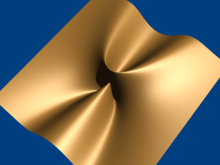
<p>[[Image:TutImgIso_11.png|Isosurface sample (cone function)]]</p> | <p>[[Image:TutImgIso_11.png|Isosurface sample (cone function)]]</p> | ||
| Line 119: | Line 119: | ||
<p><code> function { sqrt(pow(x,2) + pow(y,2) + pow(z,2)) - 2 }</code></p> | <p><code> function { sqrt(pow(x,2) + pow(y,2) + pow(z,2)) - 2 }</code></p> | ||
| + | |||
<p>[[Image:TutImgIso_12.png|Isosurface sample (sphere function)]]</p> | <p>[[Image:TutImgIso_12.png|Isosurface sample (sphere function)]]</p> | ||
| Line 128: | Line 129: | ||
<p>Allowed are:</p> | <p>Allowed are:</p> | ||
<p>User defined functions (like equations). All float expressions and operators (see section | <p>User defined functions (like equations). All float expressions and operators (see section | ||
| − | + | <!--<linkto "User-Defined Functions">User-Defined Functions</linkto>--->[[Documentation:Reference Section 2.2#User-Defined Functions|User-Defined Functions]]) which are legal | |
in POV-Ray, can be used. | in POV-Ray, can be used. | ||
| − | <br>With the equation of a sphere | + | <br>With the equation of a sphere <code>x^2+y^2+z^2 = Threshold</code> we get:</p> |
<pre> | <pre> | ||
isosurface { | isosurface { | ||
| Line 139: | Line 140: | ||
</pre> | </pre> | ||
| − | <p>Functions can be declared first (see section | + | <p>Functions can be declared first (see section <!--<linkto "User-Defined Functions">Declaring Functions</linkto>--->[[Documentation:Reference Section 2.2#User-Defined Functions|Declaring Functions]]) and |
then used in the isosurface.</p> | then used in the isosurface.</p> | ||
<pre> | <pre> | ||
| Line 196: | Line 197: | ||
<p>We can also simulate some Constructive Solid Geometry with isosurface functions. If | <p>We can also simulate some Constructive Solid Geometry with isosurface functions. If | ||
you do not know about CSG we suggest you have a look at | you do not know about CSG we suggest you have a look at | ||
| − | <!--<linkto "What is CSG?"> | + | <!--<linkto "What is CSG?">What is CSG?</linkto>--->[[Documentation:Tutorial Section 2#What is CSG?|"What is CSG?"]] or the corresponding part of the <!--<linkto "Constructive Solid Geometry">reference section</linkto>--->[[Documentation:Reference Section 4.3#Constructive Solid Geometry|reference section]] first.</p> |
<p>We will take two functions: a cylinder and a rotated box:</p> | <p>We will take two functions: a cylinder and a rotated box:</p> | ||
| Line 205: | Line 206: | ||
</pre> | </pre> | ||
| − | <p>If we combine them the following way, we get a | + | <p>If we combine them the following way, we get a <em>merge</em>:</p> |
<p><code>function { min(fn_A(x, y, z), fn_B(x, y, z)) }</code></p> | <p><code>function { min(fn_A(x, y, z), fn_B(x, y, z)) }</code></p> | ||
| Line 211: | Line 212: | ||
<p>[[Image:TutImgIso_14.png|Isosurface sample (merge)]]</p> | <p>[[Image:TutImgIso_14.png|Isosurface sample (merge)]]</p> | ||
| − | + | <p>An <em>intersection</em> can be obtained by using | |
| − | <p>An | ||
<code>max()</code> instead of <code>min()</code>:</p> | <code>max()</code> instead of <code>min()</code>:</p> | ||
| Line 219: | Line 219: | ||
<p>[[Image:TutImgIso_15.png|Isosurface sample (intersection)]]</p> | <p>[[Image:TutImgIso_15.png|Isosurface sample (intersection)]]</p> | ||
| − | <p>Of course also | + | <p>Of course also <em>difference</em> is possible, we just have to |
add a minus (-) before the second function:</p> | add a minus (-) before the second function:</p> | ||
| Line 288: | Line 288: | ||
<p>[[Image:TutImgIso_18.png|Isosurface sample (noise3d)]]</p> | <p>[[Image:TutImgIso_18.png|Isosurface sample (noise3d)]]</p> | ||
| − | <p class="Note"><strong>Note:</strong> | + | <p class="Note"><strong>Note:</strong> The <code>-0.5</code> is only there to make it match to the used threshold value of 0, the <code>f_noise3d</code> function returns values between 0 and 1.</p> |
| − | threshold value of 0, the <code>f_noise3d</code> function returns values between | ||
| − | 0 and 1.</p> | ||
<p>With this and the other functions you can generate objects similar to | <p>With this and the other functions you can generate objects similar to | ||
| Line 494: | Line 492: | ||
=====Transformations on functions===== | =====Transformations on functions===== | ||
<p> | <p> | ||
| − | Transforming an isosurface object is done like transforming any POV-Ray object. Simply use the object modifiers (scale, translate, rotate | + | Transforming an isosurface object is done like transforming any POV-Ray object. Simply use the object modifiers (scale, translate, and rotate). |
</p> | </p> | ||
| Line 519: | Line 517: | ||
Here is an overview of some useful substitutions: <br>Using a declared object P(x,y,z) | Here is an overview of some useful substitutions: <br>Using a declared object P(x,y,z) | ||
</p> | </p> | ||
| − | |||
| − | |||
<p> | <p> | ||
| Line 551: | Line 547: | ||
<pre>shear 45 degrees left gives P(x+y*tan(radians(45)), y, z)</pre> | <pre>shear 45 degrees left gives P(x+y*tan(radians(45)), y, z)</pre> | ||
| − | |||
<p><strong>Rotate</strong></p> | <p><strong>Rotate</strong></p> | ||
<p class="Note"> | <p class="Note"> | ||
| − | <strong>Note:</strong> | + | <strong>Note:</strong> These rotation substitutions work like normal POV-rotations: they already compensate for the inverse working |
| − | compensate for the inverse working | ||
</p> | </p> | ||
| Line 581: | Line 575: | ||
P(x*cos(radians(75)) + y*sin(radians(75)), | P(x*cos(radians(75)) + y*sin(radians(75)), | ||
-x*sin(radians(75)) + y*cos(radians(75)), z) | -x*sin(radians(75)) + y*cos(radians(75)), z) | ||
| − | + | </pre> | |
| − | |||
<p> | <p> | ||
| Line 601: | Line 594: | ||
<pre>flip x and y gives P(y, -x, z)</pre> | <pre>flip x and y gives P(y, -x, z)</pre> | ||
| − | |||
<p> | <p> | ||
| Line 659: | Line 651: | ||
====Poly Object==== | ====Poly Object==== | ||
<!--<indexentry "poly, tutorial">---> | <!--<indexentry "poly, tutorial">---> | ||
| − | <p>The polynomial object (and its | + | <p>The polynomial object (and its <em>shortcut</em> versions: <!--<linkto "cubic">cubic</linkto>---><code>[[Documentation:Reference Section 4.2#Poly, Cubic and Quartic|cubic]]</code>, <!--<linkto "quartic">quartic</linkto>---><code>[[Documentation:Reference Section 4.2#Poly, Cubic and Quartic|quartic]]</code> and <!--<linkto "quadric">quadric</linkto>---><code>[[Documentation:Reference Section 4.2#Quadric|quadric]]</code>) |
| − | |||
of POV-Ray is one of the most complex and | of POV-Ray is one of the most complex and | ||
mathematical primitives of the program. One could think that it is seldom | mathematical primitives of the program. One could think that it is seldom | ||
| Line 674: | Line 665: | ||
in POV-Ray.</p> | in POV-Ray.</p> | ||
| − | <p class="Note"><strong>Note: </strong>Since version 3.5, POV-Ray includes the new <code>isosurface</code> object | + | <p class="Note"><strong>Note:</strong> Since version 3.5, POV-Ray includes the new <code>isosurface</code> object |
| − | which makes the polynomial object more or less obsolete. The isosurface | + | which makes the polynomial object more or less obsolete. The isosurface is more versatile (you can specify any mathematical function, not |
| − | is more versatile (you can specify any mathematical function, not | + | just polynomials), easier to use. You can write the function as is, without needing to put values in a gigantic vector. Isosurfaces often render considerably faster than equivalent polys.</p> |
| − | just polynomials), easier to use. You can write the function as is, | ||
| − | without needing to put values in a gigantic vector. Isosurfaces | ||
| − | often render considerably faster than equivalent polys.</p> | ||
<p>However, the most mathematically oriented still like polys because | <p>However, the most mathematically oriented still like polys because | ||
| Line 686: | Line 674: | ||
are more than good enough for most applications, though.</p> | are more than good enough for most applications, though.</p> | ||
| − | <p class="Note"><strong>Note:</strong> | + | <p class="Note"><strong>Note:</strong> At it's maximum a 15th degree polynomial can be represented with the poly object. If a higher degree polynomial or other non-polynomial function has to be represented, then it is necessary to use the isosurface object.</p> |
| − | the poly object. If a higher degree polynomial or other non-polynomial function has to be represented, | ||
| − | then it is necessary to use the isosurface object.</p> | ||
=====Creating the polynomial function===== | =====Creating the polynomial function===== | ||
| Line 697: | Line 683: | ||
<p>The sphere function is:</p> | <p>The sphere function is:</p> | ||
| − | <p | + | |
| + | <p>[[Image:TutImgPolyfunc1.png|sphere function]]</p> | ||
<p>Now we have to convert this to polynomial form:</p> | <p>Now we have to convert this to polynomial form:</p> | ||
| − | <p | + | |
| + | <p>[[Image:TutImgPolyfunc2.png|sphere polynomial]]</p> | ||
<p>We will need a polynomial of the 2nd degree to represent this.</p> | <p>We will need a polynomial of the 2nd degree to represent this.</p> | ||
| Line 707: | Line 695: | ||
<p>Let's take the function:</p> | <p>Let's take the function:</p> | ||
| − | <p | + | |
| + | <p>[[Image:TutImgPolyfunc3.png|function]]</p> | ||
<p>Converting this to polynomial form we get:</p> | <p>Converting this to polynomial form we get:</p> | ||
| − | <p | + | |
| + | <p>[[Image:TutImgPolyfunc4.png|polynomial]]</p> | ||
<p>Although the highest power is 4 we will need a 5th order polynomial to | <p>Although the highest power is 4 we will need a 5th order polynomial to | ||
| Line 719: | Line 709: | ||
<p>A torus can be represented with the function:</p> | <p>A torus can be represented with the function:</p> | ||
| − | <p | + | |
| − | <p>where r<sub>1</sub> is the major radius and r<sub>2</sub> is the minor radius.</p> | + | <p>[[Image:TutImgPolyfunc5.png|torus function]]</p><p>where r<sub>1</sub> is the major radius and r<sub>2</sub> is the minor radius.</p> |
<p>Now, this is tougher to convert to polynomial form, but finally we get:</p> | <p>Now, this is tougher to convert to polynomial form, but finally we get:</p> | ||
| − | <p | + | |
| + | <p>[[Image:TutImgPolyfunc6.png|torus polynomial]]</p> | ||
<p>A 4th order polynomial is enough to represent this.</p> | <p>A 4th order polynomial is enough to represent this.</p> | ||
| − | <p class="Note"><strong>Note:</strong> | + | <p class="Note"><strong>Note:</strong> Not every function can be represented in polynomial form. Only functions that use addition (and substraction), multiplication (and division) and scalar powers (including rational powers, eg. the square root) can be represented. Also, the poly primitive supports only polynomials of the 7th degree at max.</p> |
| − | functions that use addition (and substraction), multiplication (and | ||
| − | division) and scalar powers (including rational powers, eg. the square root) | ||
| − | can be represented. Also, the poly primitive supports only | ||
| − | polynomials of the 7th degree at max.</p> | ||
<p>Converting a function to polynomial form may be a very laborious task for | <p>Converting a function to polynomial form may be a very laborious task for | ||
| Line 738: | Line 725: | ||
=====Writing the polynomial vector===== | =====Writing the polynomial vector===== | ||
<p>Now that we have the function in polynomial form, we have to write it | <p>Now that we have the function in polynomial form, we have to write it | ||
| − | in POV-Ray syntax. The syntax is specified in the in the chapters | + | in POV-Ray syntax. The syntax is specified in the in the chapters <!--<linkto "Poly, Cubic and Quartic">Poly, Cubic and Quartic</linkto>--->[[Documentation:Reference Section 4.2#Poly, Cubic and Quartic|Poly, Cubic and Quartic]] and <!--<linkto "Quadric">Quadric</linkto>--->[[Documentation:Reference Section 4.2#Quadric|Quadric]] of the SDL section. There is also a |
| − | |||
| − | |||
table in this chapter which we will be using to make the polynomial vector. It is | table in this chapter which we will be using to make the polynomial vector. It is | ||
easier to have this table printed on paper.</p> | easier to have this table printed on paper.</p> | ||
| Line 751: | Line 736: | ||
<p>Since the sphere can be represented with a polynomial of 2nd degree, we | <p>Since the sphere can be represented with a polynomial of 2nd degree, we | ||
| − | look at the row titled | + | look at the row titled <em>2nd</em> in the table. We see that it has 10 items, |
ie. we need a vector of size 10. Each item of the vector will be the factor | ie. we need a vector of size 10. Each item of the vector will be the factor | ||
of the term listed in the table.</p> | of the term listed in the table.</p> | ||
<p>The polynomial was:</p> | <p>The polynomial was:</p> | ||
| − | <p | + | |
| + | <p>[[Image:TutImgPolyfunc2.png|sphere polynomial]]</p> | ||
<p>Writing the poly in this way we get:</p> | <p>Writing the poly in this way we get:</p> | ||
| Line 792: | Line 778: | ||
} | } | ||
</pre> | </pre> | ||
| − | |||
<p>[[Image:TutImgPolypic1.png|Sphere polynomial]]</p> | <p>[[Image:TutImgPolypic1.png|Sphere polynomial]]</p> | ||
| − | <p class="Note"><strong>Note:</strong> | + | <p class="Note"><strong>Note:</strong> There is a shortcut for 2nd degree polynomials: The |
<code><!--<linkto "quadric">quadric</linkto>--->[[Documentation:Reference Section 4.2#Quadric|quadric]]</code> | <code><!--<linkto "quadric">quadric</linkto>--->[[Documentation:Reference Section 4.2#Quadric|quadric]]</code> | ||
primitive. Using a shortcut version, whenever possible, can lead to faster | primitive. Using a shortcut version, whenever possible, can lead to faster | ||
| Line 810: | Line 795: | ||
<p><strong>2)</strong> Now lets try the second one. We do it similarly, but this time we need | <p><strong>2)</strong> Now lets try the second one. We do it similarly, but this time we need | ||
| − | to look at the row titled | + | to look at the row titled <em>5th</em> in the table.</p> |
<p>The polynomial was:</p> | <p>The polynomial was:</p> | ||
| − | <p | + | |
| + | <p>[[Image:TutImgPolyfunc4.png|5th order polynomial]]</p> | ||
<p>Writing the poly primitive we get:</p> | <p>Writing the poly primitive we get:</p> | ||
| Line 860: | Line 846: | ||
<p>[[Image:TutImgPolypic2.png|5th order polynomial example]]</p> | <p>[[Image:TutImgPolypic2.png|5th order polynomial example]]</p> | ||
| − | |||
<p><strong>3)</strong> And finally the torus:</p> | <p><strong>3)</strong> And finally the torus:</p> | ||
<p>The polynomial was:</p> | <p>The polynomial was:</p> | ||
| − | <p | + | |
| + | <p>[[Image:TutImgPolyfunc6.png|torus polynomial]]</p> | ||
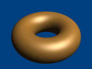
<p>And we get the proper 4th degree poly primitive:</p> | <p>And we get the proper 4th degree poly primitive:</p> | ||
| Line 891: | Line 877: | ||
<p>[[Image:TutImgPolypic3.png|Torus polynomial]]</p> | <p>[[Image:TutImgPolypic3.png|Torus polynomial]]</p> | ||
| − | |||
<p>There is a shortcut for 4th order polynomials: The | <p>There is a shortcut for 4th order polynomials: The | ||
Revision as of 16:20, 16 September 2010
|
This document is protected, so submissions, corrections and discussions should be held on this documents talk page. |
Isosurface Object
Simple functions
For the start we will choose a most simple function: x
The value of this function is exactly the current x-coordinate.
The isosurface object takes this function as a user defined function:
  isosurface {
    function { x }
    contained_by { box { -2, 2 } }
  }
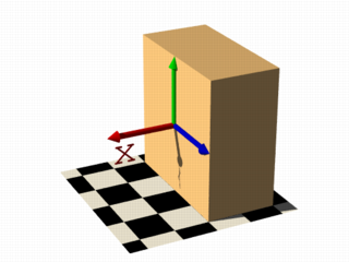
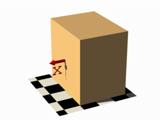
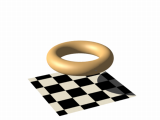
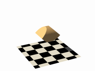
the resulting shape is fairly simple: a box.
The fact that it is a box is only caused by the container object which is required for an isosurface. You can either use a box or a sphere for this purpose.
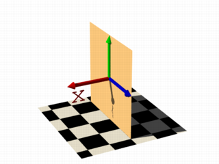
So only one side of the box is made by the function in fact. This surface is where the x-coordinate is 0 since 0 is the default threshold. There usually is no reason to change this, since it is the most common and most suggestive value, but you can specify something different by adding
threshold 1
to the isosurface definition.
As you can see, the surface is now at x-coordinate 1.
We can also remove the visible surfaces of the container object by adding the word 'open' to the isosurface definition.
For making it clearer what surfaces are the actual isosurface and what are caused by the container object, the color will be different in all the following pictures.
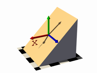
Now we replace the used function with something different:
function { x+y }
function { x+y+z }
Note: We added max_gradient 4 to the isosurface definition here, this will be explained later on.
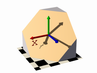
All these functions describe planes going through the origin. The function just describes the normal vector of this plane.
Several surfaces
The following two functions lead to identical results:
function { abs(x)-1 }
function { sqrt(x*x)-1 }
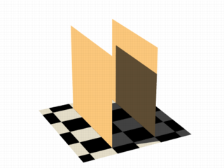
You can see that there are two planes now. The reason is that both formulas
have the same two solutions (where the function value is 0),
namely x=-1 and x=1.
We can now mix all these elements in different combinations, the results always consist of plane surfaces:
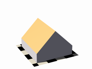
function { abs(x)-1+y }
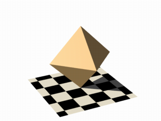
function { abs(x)+abs(y)+abs(z)-2 }
Non-linear functions
Curved surfaces of many different kinds can be achieved with non-linear functions.
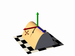
function { pow(x,2) + y }
You can see the parabolic shape caused by the square function.
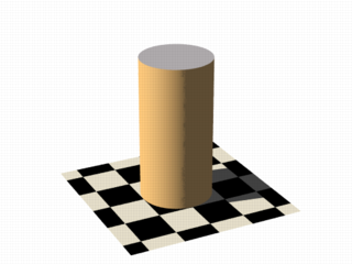
To get a cylindrical surface we can use the following function.
function { sqrt(pow(x,2) + pow(z,2)) - 1 }
In 2 dimensions it describes a circle, since it is constant in the 3rd dimension, we get a cylinder:
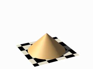
It is of course not difficult to change this into a cone, we just need to add a linear component in y-direction:
function { sqrt(pow(x,2) + pow(z,2)) + y }
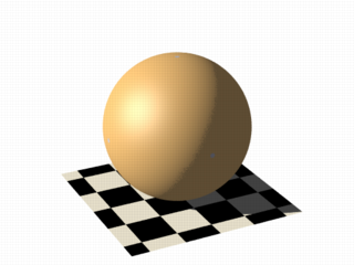
And we of course can also make a sphere:
function { sqrt(pow(x,2) + pow(y,2) + pow(z,2)) - 2 }
The 2 specifies the radius here.
Specifying functions
As we have seen, the functions used to define the isosurface are written in the function {...} block.
Allowed are:
User defined functions (like equations). All float expressions and operators (see section
User-Defined Functions) which are legal
in POV-Ray, can be used.
With the equation of a sphere x^2+y^2+z^2 = Threshold we get:
isosurface {
function {pow(x,2) + pow(y,2) + pow(z,2)}
  threshold Threshold
  ...
}
Functions can be declared first (see section Declaring Functions) and then used in the isosurface.
#declare Sphere = function {pow(x,2) + pow(y,2) + pow(z,2)}
isosurface {
  function { Sphere(x,y,z) }
  threshold Threshold
  ...
}
By default a function takes three parameters (x,y,z) and you do not have to explicitly specify
the parameter names when declaring it.
When using the identifier, the parameters must be specified.
On the other hand, if you need more or less than three parameters when declaring a function, you also have
to explicitly specify the parameter names.
#declare Sphere = function(x,y,z,Radius) {
    pow(x,2) + pow(y,2) + pow(z,2) - pow(Radius,2)
}
isosurface {
  function { Sphere(x,y,z,1) }
  ...
}
Internal functions
There are a lot of internal functions available in POV-Ray. For example
a sphere could also be generated with function { f_sphere(x, y, z, 2) }
These functions are declared in the functions.inc include file.
Most of them are more complicated and it is usually faster to use them instead of a
hand coded equivalent. See the
complete list for details.
The following makes a torus just like POV-Ray's torus object:
  #include "functions.inc"

  isosurface {
    function { f_torus(x, y, z, 1.6, 0.4) }
    contained_by { box { -2, 2 } }
  }
The 4th and 5th parameter are the major and minor radius,
just like the corresponding values in the torus{} object.
The parameters x, y and z are required, because it is a declared function. You can also declare functions yourself like it is explained in the reference section.
Combining isosurface functions
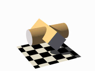
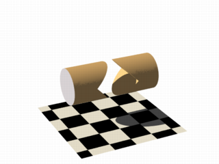
We can also simulate some Constructive Solid Geometry with isosurface functions. If you do not know about CSG we suggest you have a look at "What is CSG?" or the corresponding part of the reference section first.
We will take two functions: a cylinder and a rotated box:
  #declare fn_A = function { sqrt(pow(y,2) + pow(z,2)) - 0.8 }
  #declare fn_B = function { abs(x)+abs(y)-1 }
If we combine them the following way, we get a merge:
function { min(fn_A(x, y, z), fn_B(x, y, z)) }
An intersection can be obtained by using
max() instead of min():
function { max(fn_A(x, y, z), fn_B(x, y, z)) }
Of course also difference is possible, we just have to add a minus (-) before the second function:
function { max(fn_A(x, y, z), -fn_B(x, y, z)) }
Apart from basic CSG you can also obtain smooth transits between the different surfaces (like with the blob object)
  #declare Blob_threshold=0.01;

  isosurface {
    function {
      (1+Blob_threshold)
      -pow(Blob_threshold, fn_A(x,y,z))
      -pow(Blob_threshold, fn_B(x,y,z))
    }
    max_gradient 4
    contained_by { box { -2, 2 } }
  }
The Blob_threshold value influences the smoothness of
the transit between the shapes. a lower value leads to sharper edges.
The function for a negative blob looks like:
function{fn_A(x,y,z) + pow(Blob_threshold,(Fn_B(x,y,z) + Strength))}
Noise and pigment functions
Some of the internal functions have a random or noise-like structure
Together with the pigment functions they are one of the most powerful tools for designing isosurfaces. We can add real surface displacement to the objects rather than only normal perturbation known from the normal{} statement.
The relevant internal functions are:
f_noise3d(x,y,z)
uses the noise generator specified inglobal_settings{}and generates structures like the bozo pattern.f_noise_generator(x, y, z, noise_generator)
generates noise with a specified noise generator.f_ridged_mf(x, y, z, H, Lacunarity, Octaves, Offset, Gain, noise_generator)
generates a ridged multifractal pattern.f_ridge(x, y, z, Lambda, Octaves, Omega, Offset, Ridge, noise_generator)
generates another noise with ridges.f_hetero_mf(x, y, z, H, Lacunarity, Octaves, Offset, T, noise_generator)
generates heterogenic multifractal noise.
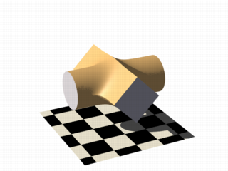
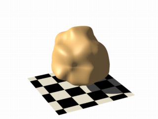
Using pure noise3d as a function results in the following picture:
function { f_noise3d(x, y, z)-0.5 }
Note: The -0.5 is only there to make it match to the used threshold value of 0, the f_noise3d function returns values between 0 and 1.
With this and the other functions you can generate objects similar to heightfields, having the advantage that a high resolution can be achieved without high memory requirements.
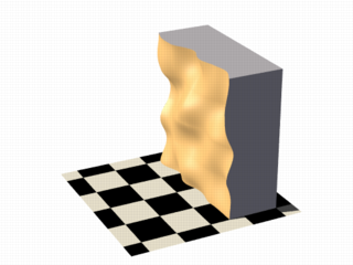
function { x + f_noise3d(0, y, z) }
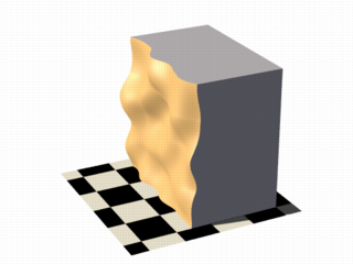
The noise function can of course also be subtracted which results in an 'inverted' version:
function { x - f_noise3d(0, y, z) }
In the last two pictures we added the noise function to a plane function. The x-parameter was set to 0 so the noise function is constant in x-direction. This way we achieve the typical heightfield structure.
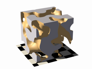
Of course we can also add noise to any other function. If the noise function is very strong this can result in several separated surfaces.
function { f_sphere(x, y, z, 1.2) - f_noise3d(x, y, z) }
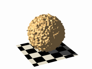
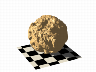
This is a noise function applied to a sphere surface, we can influence the intensity of the noise by multiplying it with a factor and change the scale by multiplying the coordinate parameters:
function { f_sphere(x, y, z, 1.6) - f_noise3d(x * 5, y * 5, z * 5) * 0.5 }
As alternative to noise functions we can also use any pigment in a function:
  #declare fn_Pigm=function {
    pigment {
      agate
      color_map {
        [0 color rgb 0]
        [1 color rgb 1]
      }
    }
  }
This function is a vector function returning a (color) vector.For use in isosurface functions they must be declared first. When using the identifier, you have to specify which component of the color vector should be used. To do this, the dot notation is used: Function(x,y,z).red.
A color vector has five components. Supported dot types to access these components are:
-
F( ).
x| F( ).u| F( ).red- to get the red value of the color vector
-
F( ).
y| F( ).v| F( ).green- to get the green value of the color vector
-
F( ).
z| F( ).blue- to get the blue value of the color vector
-
F( ).
filter| F( ).t- to get the filter value of the color vector
-
F( ).
transmit- to get the transmit value of the color vector
-
F( ).
gray- to get the gray value of the color vector
- gray value = Red*29.7% + Green*58.9% + Blue*11.4%
-
F( ).
hf- to get the height_field value of the color vector
- hf value = (Red + Green/255)*0.996093
- the .hf operator is experimental and will generate a warning.
function { f_sphere(x, y, z, 1.6)-fn_Pigm(x/2, y/2, z/2).gray*0.5 }
There are quite a lot of things possible with pigment functions, but you probably have recognized that this renders quite slow.
Conditional directives and loops
Conditional directives are allowed in functions:
#declare Rough = yes;
#include "functions.inc"
isosurface {
  function { y #if(Rough=1)-f_noise3d(x/0.5,y/0.3,z/0.4)*0.8 #end }
  ...
}
Loops can also be used in functions:
#include "functions.inc"
#declare Thr = 1/1000;
#declare Ang = radians(45);
#declare Offset = 1.5;
#declare Scale = 1.2;
#declare TrSph = function { f_sphere(x-Offset,y,z,0.7*Scale) }

function {
  (1-Thr)
  #declare A = 0;
  #while (A<8)
  -pow(Thr, TrSph(x*cos(A*Ang) + y*sin(A*Ang),
                  y*cos(A*Ang) -x*sin(A*Ang), z) )
    #declare A=A+1;
  #end
}
Note: The loops and conditionals are evaluated at parse time, not at render time.
Transformations on functions
Transforming an isosurface object is done like transforming any POV-Ray object. Simply use the object modifiers (scale, translate, and rotate).
However, when you want to transform functions within the contained_by object, you have to substitute parameters in the functions.
The results seem inverted to what you would normally expect. Here is an explanation:
Take a
Sphere(x,y,z). We know it sits at the origin because x=0. When we want it at x=2 (translating 2 units to the right) we
need to write the second equation in the same form: x-2=0
Now that both equations equal 0, we can replace
parameter x with x-2
So our Sphere(x-2, y,z) moves two units to the right.
Let's scale our Sphere 0.5 in the y direction. Default size is y=1 (one unit). We want y=0.5.
To get this
equation in the same form as the first one, we have to multiply both sides by two. y*2 = 0.5*2, which gives y*2=1
Now
we can replace the y parameter in our sphere: Sphere(x, y*2, z). This squishes the y-size of the sphere by half.
Well,
this is the general idea of substitutions.
Here is an overview of some useful substitutions:
Using a declared object P(x,y,z)
Scale
scale x : replace "x" with "x/scale" (idem other parameters)
scale x*2 gives P(x/2,y,z)
Scale Infinitely
scale x infinitely : replace "x" with "0" (idem other parameters)
scale y infinitely gives P(x,0,z)
Translate
translate x : replace "x" with "x - translation" (idem other
parameters)
translate z*3 gives P(x,y,z-3)
Shear
shear in XY-plane : replace "x" with "x + y*tan(radians(Angle))"
(idem other parameters)
shear 45 degrees left gives P(x+y*tan(radians(45)), y, z)
Rotate
Note: These rotation substitutions work like normal POV-rotations: they already compensate for the inverse working
rotate around X
: replace "y" with "z*sin(radians(Angle)) +
y*cos(radians(Angle))"
: replace "z" with "z*cos(radians(Angle)) -
y*sin(radians(Angle))"
rotate around Y
: replace "x" with "x*cos(radians(Angle)) -
z*sin(radians(Angle))"
: replace "z" with "x*sin(radians(Angle)) +
z*cos(radians(Angle))"
rotate around Z
: replace "x" with "x*cos(radians(Angle)) +
y*sin(radians(Angle))"
: replace "y" with "-x*sin(radians(Angle)) +
y*cos(radians(Angle)) "
  rotate z*75   gives:
  P(x*cos(radians(75)) + y*sin(radians(75)),
    -x*sin(radians(75)) + y*cos(radians(75)), z)
Flip
flip X - Y : replace "x" with "y" and replace "y"
with "-x"
flip Y - Z : replace "y" with "z" and replace "z"
with "-y"
flip X - Z : replace "x" with "-z" and replace "z"
with "x"
flip x and y gives P(y, -x, z)
Twist
twist N turns/unit around X
: replace "y" with "z*sin(x*2*pi*N)
+ y*cos(x*2*pi*N)"
: replace "z" with "z*cos(x*2*pi*N) -
y*sin(x*2*pi*N)"
Improving Isosurface Speed
To optimize the approximation of the isosurface and to get maximum rendering speed it is important to adapt certain values;
accuracy
The accuracy value influences how accurate the surface geometry is calculated.
Lower values lead to a more precise, but slower result.
The default value of 0.001 is fairly low. We used this value in all the
previous samples, but often you can raise this quite a
lot and thereby make things faster.
max_gradient
For finding the actual surface it is important for POV-Ray to know the
maximum gradient of the function, meaning how fast the function value changes.
We can specify a value with the max_gradient keyword. Lower
max_gradient values lead to faster rendering, but if the specified value is
below the actual maximum gradient of the function, there can be holes or
other artefacts in the surface.
For the same reason functions with infinite gradient should not be used.
This applies for pigment functions with brick or checker pattern for example.
You should also be careful when using select() in isosurface
functions because of this.
If the real maximum gradient differs too much from the specified value
POV-Ray prints a warning together with the found maximum gradient.
It is usually sufficient to use this number for the max_gradient
parameter to get fast and correct results.
POV-Ray can also dynamically change the max_gradient when you
specify evaluate with 3 parameters the isosurface definition.
Concerning the details on this and other things see the
evaluate in the reference section.
contained_by
Make sure your contained_by 'object' fits as tightly as possible. An oversized container can
sky-rocket the render time.
When the container has a lot of empty space around the actual isosurface, POV-Ray has
to do a lot of superfluous sampling: especially with complex functions this can become very time consuming. On top of
this, the max_gradient needed to get a proper surface will also increase rapidly (almost proportional to
the oversize!).
You could use a transparent copy of the container (using exactly the same transformations) to
check how it fits. Getting the min_extent and max_extent of the isosurface
is not useful because it only gives the extent of the container and not of the actual isosurface.
Poly Object
The polynomial object (and its shortcut versions: cubic, quartic and quadric)
of POV-Ray is one of the most complex and
mathematical primitives of the program. One could think that it is seldom
used and more or less obsolete, but we have to remember that for example
the torus primitive is just a shortcut for the equivalent quartic, which
is just a shortcut for the equivalent poly object. Polys are, however, seldom
used in scenes due to the fact that they are so difficult to define and
it is far from trivial to get the desired shape with just a polynomial
equation. It is mostly used by the most mathematically oriented POV-Ray
users.
This tutorial explains the process of making a polynomial object in POV-Ray.
Note: Since version 3.5, POV-Ray includes the new isosurface object
which makes the polynomial object more or less obsolete. The isosurface is more versatile (you can specify any mathematical function, not
just polynomials), easier to use. You can write the function as is, without needing to put values in a gigantic vector. Isosurfaces often render considerably faster than equivalent polys.
However, the most mathematically oriented still like polys because isosurfaces are calculated just by approximating the right value, while the poly is calculated in a mathematically exact way. Usually isosurfaces are more than good enough for most applications, though.
Note: At it's maximum a 15th degree polynomial can be represented with the poly object. If a higher degree polynomial or other non-polynomial function has to be represented, then it is necessary to use the isosurface object.
Creating the polynomial function
The first step is to create the polynomial function to be represented. You will need some (high-school level) mathematical knowledge for this.
1) Let's start with an easy example: A sphere.
The sphere function is:
Now we have to convert this to polynomial form:
We will need a polynomial of the 2nd degree to represent this.
2) A more elaborated example:
Let's take the function:
Converting this to polynomial form we get:
Although the highest power is 4 we will need a 5th order polynomial to represent this function (because we cannot represent y4z with a 4th order polynomial).
3) And since we talked about the torus, let's also take it as an example.
A torus can be represented with the function:
where r1 is the major radius and r2 is the minor radius.
Now, this is tougher to convert to polynomial form, but finally we get:
A 4th order polynomial is enough to represent this.
Note: Not every function can be represented in polynomial form. Only functions that use addition (and substraction), multiplication (and division) and scalar powers (including rational powers, eg. the square root) can be represented. Also, the poly primitive supports only polynomials of the 7th degree at max.
Converting a function to polynomial form may be a very laborious task for certain functions. Some mathematical programs are very helpful in this matter.
Writing the polynomial vector
Now that we have the function in polynomial form, we have to write it in POV-Ray syntax. The syntax is specified in the in the chapters Poly, Cubic and Quartic and Quadric of the SDL section. There is also a table in this chapter which we will be using to make the polynomial vector. It is easier to have this table printed on paper.
Note: It is also possible to make a little program with your favorite programming language which will print the poly vector from the polynomial function, but making a program like this is up to you.
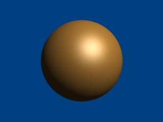
1) Let's start with the easy one, ie. the sphere.
Since the sphere can be represented with a polynomial of 2nd degree, we look at the row titled 2nd in the table. We see that it has 10 items, ie. we need a vector of size 10. Each item of the vector will be the factor of the term listed in the table.
The polynomial was:
Writing the poly in this way we get:
#declare Radius=1;
poly
{ 2,
  <1,0,0,0,1,
   0,0,1,0,-Radius*Radius>
}
Put each group of factors (separated with lines in the table) in their own lines.
In the table we see that the first item is the factor for x2, which is 1 in the function. The next item is xy. Since it is not in the function, its factor is 0. Likewise the next item, which is xz. And so on. The last item is the scalar term, which is in this case -r2.
If we make a proper scene and render it, we get:
camera { location y*4-z*5 look_at 0 angle 35 }
light_source { <100,200,-50> 1 }
background { rgb <0,.25,.5> }

#declare Radius=1;
poly
{ 2,
  <1,0,0,0,1,
   0,0,1,0,-Radius*Radius>
  pigment { rgb <1,.7,.3> } finish { specular .5 }
}
Note: There is a shortcut for 2nd degree polynomials: The
quadric
primitive. Using a shortcut version, whenever possible, can lead to faster
renderings. We can write the sphere code described above in the following
way:
quadric
{ <1,1,1>, <0,0,0>, <0,0,0>, -Radius*Radius
  pigment { rgb <1,.7,.3> } finish { specular .5 }
}
2) Now lets try the second one. We do it similarly, but this time we need to look at the row titled 5th in the table.
The polynomial was:
Writing the poly primitive we get:
poly
{ 5,
  <0,0,0,0,0,
   0,0,0,0,0,
   0,0,0,0,0,
   0,0,0,1,0,
   0,0,0,0,0,
   -2,0,0,0,0,
   0,0,0,0,0,
   0,1,0,0,0,
   0,0,0,0,0,
   0,0,0,0,0,
   0,0,0,0,0,0>
}
With the proper scene we get:
camera { location <8,20,-10>*.7 look_at x*.01 angle 35 }
light_source { <100,200,20> 1 }
background { rgb <0,.25,.5> }

poly
{ 5,
  <0,0,0,0,0,
   0,0,0,0,0,
   0,0,0,0,0,
   0,0,0,1,0,
   0,0,0,0,0,
   -2,0,0,0,0,
   0,0,0,0,0,
   0,1,0,0,0,
   0,0,0,0,0,
   0,0,0,0,0,
   0,0,0,0,0,0>
  clipped_by { box { <-4,-4,-1><4,4,1> } }
  bounded_by { clipped_by }
  pigment { rgb <1,.7,.3> } finish { specular .5 }
  rotate <0,90,-90>
}
3) And finally the torus:
The polynomial was:
And we get the proper 4th degree poly primitive:
camera { location y*4-z*5 look_at 0 angle 35 }
light_source { <100,200,-50> 1 }
background { rgb <0,.25,.5> }

#declare r1=1;
#declare r2=.5;
poly
{ 4,
  <1,0,0,0,2,
   0,0,2,0,-2*(r1*r1+r2*r2),
   0,0,0,0,0,
   0,0,0,0,0,
   1,0,0,2,0,
   2*(r1*r1-r2*r2),0,0,0,0,
   1,0,-2*(r1*r1+r2*r2),0,pow(r1,4)+pow(r2,4)-2*r1*r1*r2*r2>
  pigment { rgb <1,.7,.3> } finish { specular .5 }
}
When rendered we get:
There is a shortcut for 4th order polynomials: The
quartic primitive.
We can write the torus like this:
quartic
{ <1,0,0,0,2,
   0,0,2,0,-2*(r1*r1+r2*r2),
   0,0,0,0,0,
   0,0,0,0,0,
   1,0,0,2,0,
   2*(r1*r1-r2*r2),0,0,0,0,
   1,0,-2*(r1*r1+r2*r2),0,pow(r1,4)+pow(r2,4)-2*r1*r1*r2*r2>
  pigment { rgb <1,.7,.3> } finish { specular .5 }
}
| Isosurface Object | Superquadric Ellipsoid Object |
|
This document is protected, so submissions, corrections and discussions should be held on this documents talk page. |
