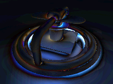
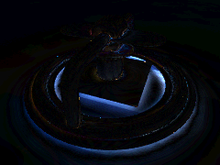
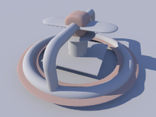
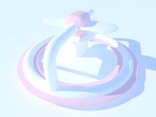
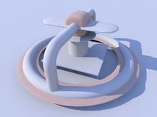
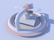
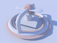
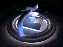
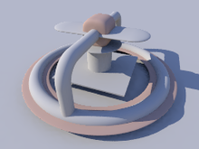
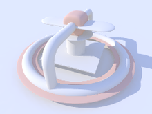
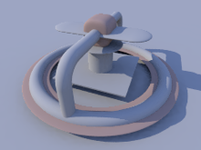
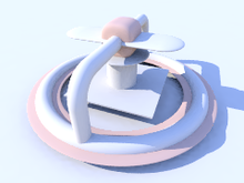
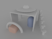
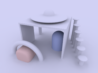
Documentation Talk:Tutorial Section 3.7

Radiosity with conventional lighting

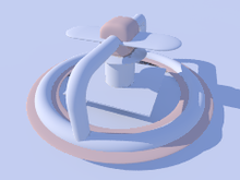
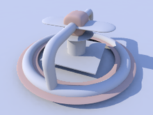
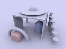
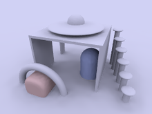
This section will introduce you to the technique of combining conventional and radiosity lighting. In this part of the tutorial, we'll be using basically the same sample scene that's located at ~/scenes/radiosity/radiosity2.pov, however by changing various radiosity parameters, we'll be able to explore the effects that those changes can have on the scenes appearance and in some cases the render time. Later on, in this tutorial, you can find examples of pure radiosity illumination.

Note: Unless otherwise stated all the images in this section were rendered with the following radiosity settings:

  global_settings {
    radiosity {
      pretrace_start 0.08
      pretrace_end   0.01
      count 150
      nearest_count 10
      error_bound 0.5
      recursion_limit 3
      low_error_factor 0.5
      gray_threshold 0.0
      minimum_reuse 0.005
      maximum_reuse 0.2
      brightness 1
      adc_bailout 0.005
    }
  }

Finally, a few more things about the scene setup. All objects except the sky have diffuse 0.65 and emission 0 in their finish block. The sky sphere has a bright blue pigment (what a surprise) with diffuse 0 and emission 1.0 as finish attributes.

Note: If using the sky_sphere object, which does not support the finish keyword, instead of a sphere object that does, you will need define a #default finish in order to affect it's finish properties.

For example:

#default {finish { diffuse 0 emission 1 }}

Hint: You can easily turn radiosity on/off with the use of a conditional statement.

#declare UseRad = yes;

  global_settings {
  #if (UseRad)
    radiosity {
      rad settings ...
    }
  #end
  }

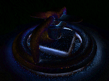
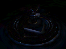
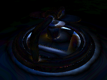
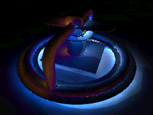
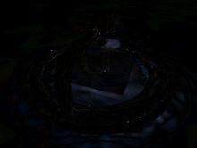
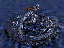
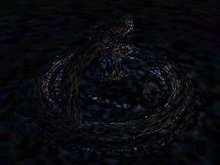
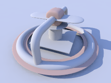
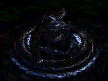
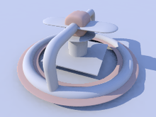
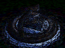
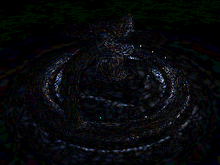
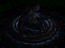
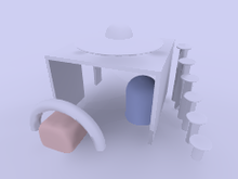
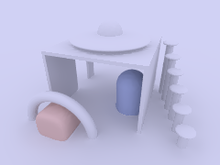
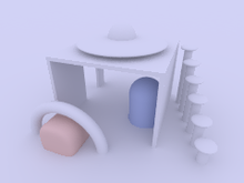
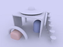
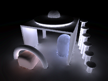
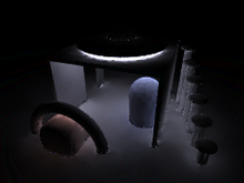
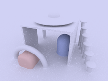
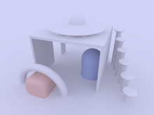
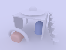
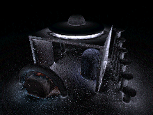
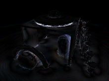
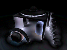
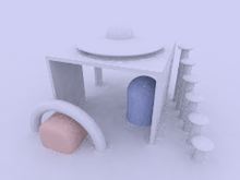
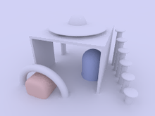
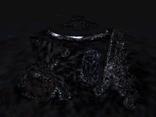
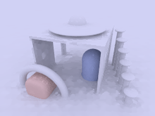
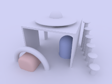
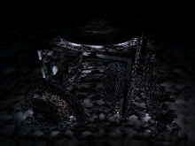
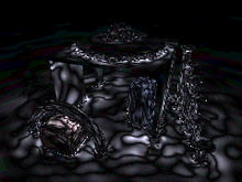
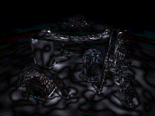
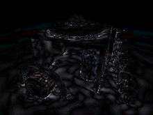
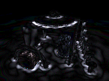
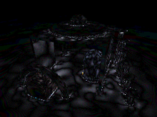
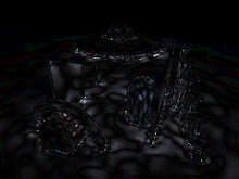
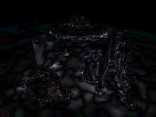
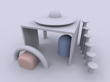
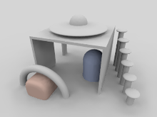
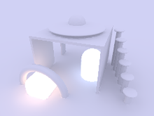
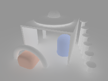
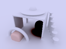
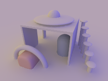
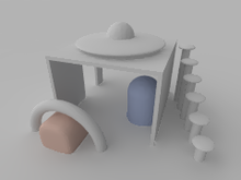
OK, let's get started! In this set of images we first have the scene as it should appear without radiosity, in other words the radiosity block has been removed, next with the settings noted above, and finally an image showing the difference between the two. Looking at the difference image, you can see that radiosity greatly affects the shadowed areas when applied in combination with conventional lighting.

Note: The use of emission 1 in the finish block of the blue sky is what gives the bluish touch of the whole scene in the radiosity version, as it functions as kind of a diffuse light source.

no radiosity	radiosity	difference w/o radiosity

Radiosity is a highly tunable process, and it comes equipped with a variety of tunable parameters that make it easy to strike a balance between quality and rendering speed. However, as with most things, higher quality means more render time. Patience is a virtue.

For instance, let's examine our test object with default settings, with our reference settings, and finally with some maddeningly high-quality settings. For comparison, below each image you can see the difference to the high-quality version.

default settings	high-quality render	tutorial reference settings
default settings difference		tutorial reference settings difference

Changing the brightness changes the intensity of radiosity effects. Theoretically specifying brightness 0 would be the same as without radiosity, however in practice POV-Ray doesn't accept a zero value. As a rule brightness 1 should work correctly in most cases. If the effects are too strong you can reduce this, though this is not recommended, as it's usually an indication that your textures are too bright and your illumination too dim. Larger values can lead to quite strange results in most cases.

brightness 0.5	brightness 1.0	brightness 2.0

The recursion_limit setting primarily affects the brightness of shadows, nooks and corners. The following group of images show the results of setting this parameter to 1, 2 and 5 respectively ...

recursion_limit 1	recursion_limit 2	recursion_limit 5

... while this next grouping shows the difference when compared to our reference setting of recursion_limit 3. As you can see, values higher than 3 do not lead to any better results in such a quite simple scene. In most cases values of 1 or 2 are sufficient, especially for outdoor scenes.

recursion_limit 1 difference	recursion_limit 2 difference	recursion_limit 5 difference

The error_bound setting mainly affects the structures of the shadows. Values larger than the default of 1.8 do not have much effect, they make the shadows even flatter. Extremely low values can lead to very good results, but the rendering time can become very long, and you may need to modify other parameters to avoid a grainy appearance.

error_bound 0.01	error_bound 1.0	error_bound 1.8
error_bound 0.01 difference	error_bound 1.0 difference	error_bound 1.8 difference

Somewhat related to error_bound is low_error_factor. It reduces error_bound setting during the pretrace phase, changing this can be useful to eliminate artifacts. The difference images used the low_error_factor 0.5 case for comparison.

low_error_factor 0.01	low_error_factor 0.5	low_error_factor 1.0
low_error_factor 0.01 difference		low_error_factor 1.0 difference

This next sequence of images illustrate the effect of count. It is a general quality and accuracy parameter leading to higher quality and slower rendering at higher values. Keep in mind that higher count isn't necessarily a cure-for-all when it comes to quality. The difference images were compared to a count 150 case.

Note: Until otherwise noted the following settings are being used to emphasize the effects of the next parameters we'll be examining.

• recursion_limit 1
• error_bound 0.2
• low_error_factor 1.0

count 2	count 35 (default)	count 1000
count 2 difference	count 35 difference	count 1000 difference

Another parameter that affects quality is nearest_count. You can use values ranging from 1 to 20 the default is 5. Just like count, higher values can lead to less artifacts and smoother appearance but slower rendering. The nearest_count setting also accepts a second parameter, which activates adaptive pretrace, providing a good means of speeding up pretrace without significant loss of quality (not shown here) the value must be smaller than the first parameter (e.g. nearest_count 20,10). When set, POV-Ray will stop pretracing individual areas of the image where the average sample density already satisfies this second value, thereby avoiding tracing low-detail areas over and over again for little gain, while still being able to drill down deep into high-detail areas. A setting of nearest_count 10 was used for the comparison.

nearest_count 1	nearest_count 5 (default)	nearest_count 20
nearest_count 1 difference	nearest_count 5 difference	nearest_count 20 difference

minimum_reuse influences at which minimum distance previous radiosity samples are always reused during calculation, affecting quality and smoothness in nooks and corners. Higher values generally give a smoother appearance, at the cost of corner detail, while lower values may cause corners to look splotchy unless the other parameters (most notably count and nearest_count) are set for higher quality as well.

As minimum_reuse must be lower than maximum_reuse, to avoid a parse error with the highest setting we're using maximum_reuse 0.4 and the minimum_reuse 0.005 case, was used for the comparison with these next three images.

minimum_reuse 0.2	minimum_reuse 0.005	minimum_reuse 0.015
minimum_reuse 0.2 difference		minimum_reuse 0.015 difference

Another important setting is pretrace_end. It specifies how many pretrace steps are calculated and thereby strongly influences the speed. Usually lower values lead to better quality, but it is important to keep this in good relation to error_bound.

pretrace_end 0.2	pretrace_end 0.01	pretrace_end 0.001
pretrace_end 0.2		pretrace_end 0.001

Normally in the final trace no additional radiosity samples are taken unless absolutely needed. You can change this by adding always_sample on allowing you to increase pretrace_end to speed up rendering. Note however that this is very prone to artifacts such as visible render block boundaries and horizontal "smearing", so it is usually only useful for test renders. You should also use a low setting for nearest_count, or you may actually increase the rendering time, and the probability of getting the mentioned artifacts!.

always_sample off	always_sample on difference	always_sample on

The effect of max_sample is similar to brightness. It does not reduce the radiosity effect in general but weakens samples with brightness above the specified value.

max_sample 0.5	max_sample 0.8	max_sample not set (default)

You can strongly affect things with an object's finish attributes. In fact that is the most important thing about radiosity. Normal objects should have an emission 0 (the default) finish. Objects with an emission setting greater than zero actually act as light sources in radiosity scenes. Remember that the default finish values used until now were diffuse 0.65 and emission 0.

diffuse 0.65 emission 0.2	diffuse 0.4 emission 0	diffuse 1.0 emission 0

Finally you can vary the sky in outdoor radiosity scenes. In all these examples it is implemented with a sphere object. finish { emission 1 diffuse 0 } and the pigment of the original sample scene were used until now. The following images show some variations.

emission 0 diffuse 1	emission 0 diffuse 0 (no sky)	rgb <1,0.8,0> to blue 1 gradient

Radiosity without conventional lighting

Radiosity also allows us to have scenes without conventional light sources. What's left is a situation that's similar to what you'd expect on a cloudy day where the light comes from no specific direction but from the whole sky.

Reminder: The following settings are still in effect.

• recursion_limit 1
• error_bound 0.2
• low_error_factor 1.0

You can see that when the light source is removed the whole image takes on a noticeable blue tint. That's because the scene is now illuminated by our sky object, which in this case happens to be blue. Later on you'll see how varying the color of the sky influences the appearance of the scene.

with light source	without light source

Note: We'll be using the sample scene ~/scenes/radiosity/radiosity3.pov for the rest of this tutorial.

This next series of images show our new test object with the default settings, then our reference settings, and lastly those maddeningly high-quality settings we used earlier. Notice that with the default settings, the image looks much worse than in the first part of this tutorial. The reason being, those settings were mainly selected for use with a conventionally lit scene. Keep in mind, radiosity-only scenes are less forgiving of low-quality settings.

Note: As a reminder you might want to refer back to the reference settings used at the beginning of this tutorial.

default settings	tutorial reference settings	maddeningly high-quality settings

The following images demonstrate the effect of different settings for recursion_limit.

recursion_limit 1	recursion_limit 3	recursion_limit 2
recursion_limit 1 difference		recursion_limit 2 difference

The next three images show the effect of error_bound. In scenes without light sources, this is even more important than than scenes that do. Good values mostly depend on the scenery and the other settings, lower values do not necessarily lead to better results. Note that we're using our error_bound 0.5 image as reference.

error_bound 0.01	error_bound 1.0	error_bound 1.8
error_bound 0.01 difference	error_bound 1.0 difference	error_bound 1.8 difference

If there are artifacts it often helps to increase count, it does affect quality in general and often helps removing them, the following three images use error_bound 0.2.

count 2	count 50	count 200
count 35 difference		count 150 difference

As can be seen upon closer inspection however, this is no magic cure-all, some bright speckles remain even with extremely high count values.

In this case, the reason is that the pretrace is simply too short to provide the number of samples we aim for. This is a job for pretrace_end: Together with pretrace_start it specifies how many pretrace steps are done, and how high their resolution is. Lower values of pretrace_end lead to more pretrace steps and more accurate results but also to significantly slower rendering.

We're still using error_bound 0.1 for these images.

pretrace_end 0.4	pretrace_end 0.01	pretrace_end 0.001
pretrace_end 0.4 difference		pretrace_end 0.001 difference

This next sequence shows the effect of nearest_count, the difference is not very strong, but larger values always lead to better results, the maximum is 20. We'll be using error_bound 0.5 again, but also the following modifications to emphasize the effect.

• recursion_limit 1
• low_error_factor 1.0
• pretrace_end 0.001

Note: From now on we'll stick to these values.

nearest_count 2	nearest_count 5 (default)	nearest_count 20
nearest_count 2 difference	nearest_count 5 difference	nearest_count 20 difference

The minimum_reuse is a geometric value related to the size of the render in pixels and affects whether previous radiosity calculations are reused at a new point. Lower values lead to more often and therefore more accurate calculations, but care must be taken to balance this setting with the others. The minimum_reuse 0.05 was used for the comparison.

minimum_reuse 0.1	minimum_reuse 0.05 (default)	minimum_reuse 0.015
minimum_reuse 0.1 difference		minimum_reuse 0.015 difference

In most cases it is not necessary to change the low_error_factor. This setting reduces the error_bound value during the final pretrace step. Changing this value can sometimes help to remove persistent artifacts.

low_error_factor 0.01	low_error_factor 0.5 (default)	low_error_factor 1.0
low_error_factor 0.01 difference		low_error_factor 1.0 difference

The gray_threshold setting reduces the color in the radiosity calculations. As mentioned above the blue sky affects the color of the whole scene when radiosity is calculated. To reduce this coloring effect without affecting radiosity in general you can increase gray_threshold. A value of 1.0 means no color in radiosity at all.

gray_threshold 0.0 (default)	gray_threshold 0.5	gray_threshold 1.0

It is worth experimenting with the things affecting radiosity to get some feeling for how things work. The next 3 images show some more experiments. We're back with the original reference settings from now on.

emission 3 for two objects	all objects emission 0.3 sky gets 0	emission -3 for one object

Finally you can strongly change the appearance of the whole scene with the sky's texture. The following images give some examples.

rgb <1,0.8,0> to blue gradient	light-dark gradient from left-right	light-dark gradient from bottom-top

Really good results mostly depend on the single situation and how the scene is meant to look. We used these settings listed below, to get this example of a higher quality render of our test object. It's important to remember that requirements can be much different from scene to scene.
	higher quality radiosity scene

  global_settings {
    radiosity {
      pretrace_start 0.128
      pretrace_end   0.002
      count 500
      nearest_count 20
      error_bound 0.5
      recursion_limit 2
      low_error_factor 1.0
      gray_threshold 0.0
      minimum_reuse 0.005
      maximum_reuse 0.1
      brightness 1
      adc_bailout 0.005
    }
  }

Normals and Radiosity

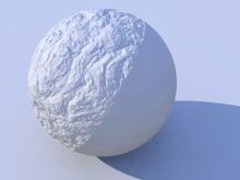
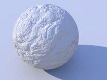
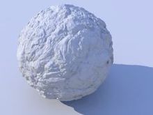
When using a normal statement in combination with radiosity lighting, you will see that the shadowed parts of the objects are totally smooth, no matter how strong the normals are made. The reason is that POV-Ray by default does not take the normal into account when calculating radiosity. You can easily change this by adding normal on to the radiosity block. Be aware that this can slow things down quite a bit and will require more memory, however it usually leads to more realistic results.

When using normals you should also remember that they are only faked irregularities and do not generate real geometric disturbances of the surface. A more realistic approach is using an isosurface with a pigment function, but this can quickly lead to increased render times.

As you can see with this next series of images, the isosurface version does not have the same smooth-like appearance to it's circumference, as compared to the first two images. Notice that it also has a more realistic shadow-line.

normal off (default)	normal on	isosurface