Documentation:Tutorial Section 3.7

This document is protected, so submissions, corrections and discussions should be held on this documents talk page.

Simple Media Tutorial

Multiple medias inside the same object

Emitting media works well with dark backgrounds. Absorbing media works well for light backgrounds. But what if we want a media which works with both type of backgrounds?

One solution for this is to use both types of medias inside the same object. This is possible in POV-Ray.

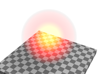
Let's take the very first example, which did not work well with the white background, and add a slightly absorbing media to the sphere:

 sphere
 { 0,1 pigment { rgbt 1 } hollow
   interior
   { media
     { emission 1
       density
       { spherical density_map
         { [0 rgb 0]
           [0.4 rgb <1,0,0>]
           [0.8 rgb <1,1,0>]
           [1 rgb 1]
         }
       }
     }
     media
     { absorption 0.2
     }
   }
 }

This will make the sphere not only add light to the rays passing through it, but also substract.

Multiple medias in the same object can be used for several other effects as well.

Media and transformations

The density of a media can be modified with any pattern modifier, such as turbulence, scale, etc. This is a very powerful tool for making diverse effects.

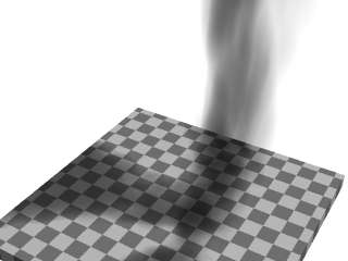
As an example, let's make an absorbing media which looks like smoke. For this we take the absorbing media example and modify the sphere like this:

 sphere
 { 0,1.5 pigment { rgbt 1 } hollow
   interior
   { media
     { absorption 7
       density
       { spherical density_map
         { [0 rgb 0]
           [0.5 rgb 0]
           [0.7 rgb .5]
           [1 rgb 1]
         }
         scale 1/2
         warp { turbulence 0.5 }
         scale 2
       }
     }
   }
   scale <1.5,6,1.5> translate y
 }

A couple of notes:

The radius of the sphere is now a bit bigger than 1 because the turbulent pattern tends to take more space.

The absorption color can be larger than 1, making the absorption stronger and the smoke darker.

Note: When you scale an object containing media the media density is not scaled accordingly. This means that if you for example scale a container object larger the rays will pass through more media than before, giving a stronger result. If you want to keep the same media effect with the larger object, you will need to divide the color of the media by the scaling amount.

The question of whether the program should scale the density of the media with the object is a question of interpretation: For example, if you have a glass of colored water, a larger glass of colored water will be more colored because the light travels a larger distance. This is how POV-Ray behaves. Sometimes, however, the object needs to be scaled so that the media does not change; in this case the media color needs to be scaled inversely.

A more advanced example of scattering media

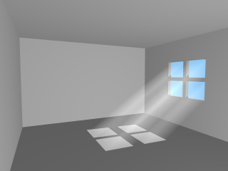
For a bit more advanced example of scattering media, let's make a room with a window and a light source illuminating from outside the room. The room contains scattering media, thus making the light beam coming through the window visible.

 global_settings { assumed_gamma 1 }
 camera { location <14.9, 1, -8> look_at -z angle 70 }
 light_source { <10,100,150>, 1 }
 background { rgb <0.3, 0.6, 0.9> }

 // A dim light source inside the room which does not
 // interact with media so that we can see the room:
 light_source { <14, -5, 2>, 0.5 media_interaction off }

 // Room
 union
 { difference
   { box { <-11, -7, -11>, <16, 7, 10.5> }
     box { <-10, -6, -10>, <15, 6, 10> }
     box { <-4, -2, 9.9>, <2, 3, 10.6> }
   }
   box { <-1.25, -2, 10>, <-0.75, 3, 10.5> }
   box { <-4, 0.25, 10>, <2, 0.75, 10.5> }
   pigment { rgb 1 }
 }
 
 // Scattering media box:
 box
 { <-5, -6.5, -10.5>, <3, 6.5, 10.25>
   pigment { rgbt 1 } hollow
   interior
   { media
     { scattering { 1, 0.07 extinction 0.01 }
       samples 30
     }
   }
 }

As suggested previously, the scattering color and extinction values were adjusted until the image looked good. In this kind of scene usually very small values are needed.

Note how the container box is quite smaller than the room itself. Container boxes should always be sized as minimally as possible. If the box were as big as the room much higher values for samples would be needed for a good result, thus resulting in a much slower rendering.

Media and photons

The photon mapping technique can be used in POV-Ray for making stunningly beautiful images with light reflecting and refracting from objects. By default, however, reflected and refracted light does not affect media. Making photons interact with media can be turned on with the media keyword in the photons block inside global_settings.

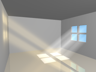
To visualize this, let's make the floor of our room reflective so that it will reflect the beam of light coming from the window.

Firstly, due to how photons work, we need to specify photons { pass_through } in our scattering media container box so that photons will pass through its surfaces.

Secondly, we will want to turn photons off for our fill-light since it's there only for us to see the interior of the room and not for the actual lighting effect. This can be done by specifying photons { reflection off } in that light source.

Thirdly, we need to set up the photons and add a reflective floor to the room. Let's make the reflection colored for extra effect:

 global_settings
 { photons
   { count 20000
     media 100
   }
 }
 
 // Reflective floor:
 box
 { <-10, -5.99, -10>, <15, -6, 10>
   pigment { rgb 1 }
   finish { reflection <0.5, 0.4, 0.2> }
   photons { target reflection on }
 }

With all these fancy effects the render times start becoming quite high, but unfortunately this is a price which has to be paid for such effects.

Radiosity

Introduction

Radiosity is a lighting technique to simulate the diffuse exchange of radiation between the objects of a scene. With a raytracer like POV-Ray, normally only the direct influence of light sources on the objects can be calculated, all shadowed parts look totally flat. Radiosity can help to overcome this limitation. More details on the technical aspects can be found in the reference section.

To enable radiosity, you have to add a radiosity block to the global_settings in your POV-Ray scene file. Radiosity is more accurate than simplistic ambient light but it takes much longer to compute, so it can be useful to switch off radiosity during scene development. You can use a declared constant or an INI-file constant and an #if statement to do this:

  #declare RAD = off;

  global_settings {
     #if(RAD)
        radiosity {
           ...
        }
     #end
  }

Most important for radiosity are the ambient and diffuse finish components of the objects. Their effect differs quite greatly from a conventionally lit scene.

ambient: specifies the amount of light emitted by the object. This is the basis for radiosity without conventional lighting but also in scenes with light sources this can be important. Since most materials do not actually emit light, the default value of 0.1 is too high in most cases. You can also change ambient_light to influence this.
diffuse: influences the amount of diffuse reflection of incoming light. In a radiosity scene this does not only mean the direct appearance of the surface but also how much other objects are illuminated by indirect light from this surface.

Radiosity with conventional lighting

The pictures here introduce combined conventional/radiosity lighting. Later on you can also find examples for pure radiosity illumination.

The following settings are default, the result will be the same with an empty radiosity block:

  global_settings {
    radiosity {
      pretrace_start 0.08
      pretrace_end   0.04
      count 35

      nearest_count 5
      error_bound 1.8
      recursion_limit 3

      low_error_factor 0.5
      gray_threshold 0.0
      minimum_reuse 0.015
      brightness 1

      adc_bailout 0.01/2
    }
  }

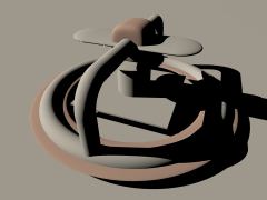
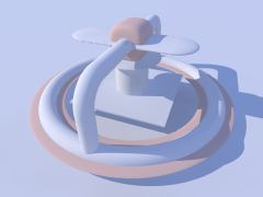
The following pictures are rendered with default settings and are made to introduce the sample scene.

All objects except the sky have an ambient finish of 0.

The ambient 1 finish of the blue sky makes it functioning as some kind of diffuse light source. This leads to a bluish touch of the whole scene in the radiosity version.

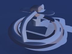You can see that radiosity greatly affects the shadowed parts when applied combined with conventional lighting.

Changing brightness changes the intensity of radiosity effects. brightness 0 would be the same as without radiosity. brightness 1 should work correctly in most cases, if effects are too strong you can reduce this. Larger values lead to quite strange results in most cases.

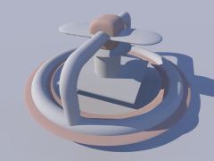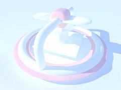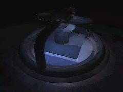
Changing the recursion_limit value leads to the following results, second line are difference to default (recursion_limit 3):

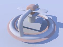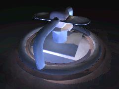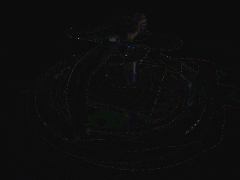You can see that higher values than the default of 3 do not lead to much better results in such a quite simple scene. In most cases values of 1 or 2 are sufficient.

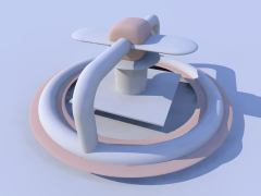
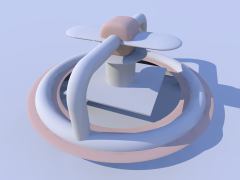
The error_bound value mainly affects the structures of the shadows. Values larger than the default of 1.8 do not have much effect, they make the shadows even flatter. Extremely low values can lead to very good results, but the rendering time can become very long. For the following samples recursion_limit 1 is used.

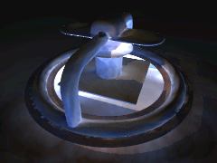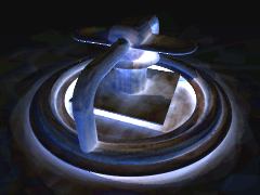
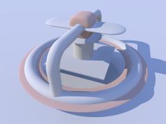
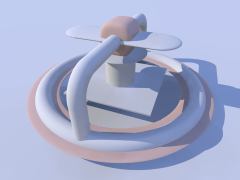
Somewhat related to error_bound is low_error_factor. It reduces error_bound during the last pretrace step. Changing this can be useful to eliminate artefacts.

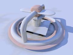
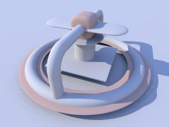
The next samples use recursion_limit 1 and error_bound 0.2. These 3 pictures illustrate the effect of count. It is a general quality and accuracy parameter leading to higher quality and slower rendering at higher values.

Another parameter that affects quality is nearest_count. You can use values from 1 to 20, default is 5:

Again higher values lead to less artefacts and smoother appearance but slower rendering.

minimum_reuse influences whether previous radiosity samples are reused during calculation. It also affects quality and smoothness.

Another important value is pretrace_end. It specifies how many pretrace steps are calculated and thereby strongly influences the speed. Usually lower values lead to better quality, but it is important to keep this in good relation to error_bound.

Strongly related to pretrace_end is always_sample. Normally even in the final trace additional radiosity samples are taken. You can avoid this by adding always_sample off. That is especially useful if you load previously calculated radiosity data with load_file.

The effect of max_sample is similar to brightness. It does not reduce the radiosity effect in general but weakens samples with brightness above the specified value.

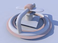
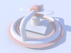
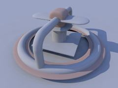
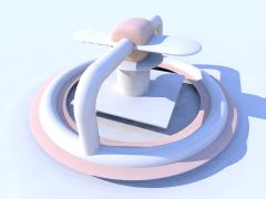
You can strongly affect things with the objects' finishes. In fact that is the most important thing about radiosity. Normal objects should have ambient finish 0 which is not default in POV-Ray and therefore needs to be specified. Objects with ambient > 0 actually emit light.

Default finish values used until now are diffuse 0.65 ambient 0.

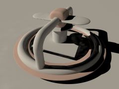
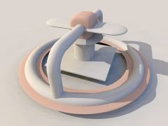
Finally you can vary the sky in outdoor radiosity scenes. In all these examples it is implemented with a sphere object. finish { ambient 1 diffuse 0 } was used until now. The following pictures show some variations:

Radiosity without conventional lighting

You can also leave out all light sources and have pure radiosity lighting. The situation then is similar to a cloudy day outside, when the light comes from no specific direction but from the whole sky.

The following 2 pictures show what changes with the scene used in part 1, when the light source is removed. (default radiosity, but recursion_limit 1 and error_bound 0.2)

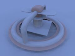You can see that when the light source is removed the whole picture becomes very blue, because the scene is illuminated by a blue sky, while on a cloudy day, the color of the sky should be somewhere between grey and white.

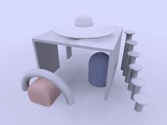
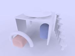
The following pictures show the sample scene used in this part with different settings for recursion_limit (everything else default settings).

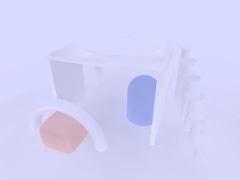This looks much worse than in the first part, because the default settings are mainly selected for use with conventional light sources.

The next three pictures show the effect of error_bound. (recursion_limit is 1 here) Without light sources, this is even more important than with, good values mostly depend on the scenery and the other settings, lower values do not necessarily lead to better results.

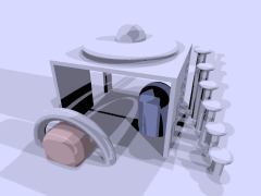
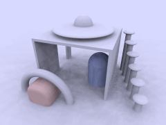
If there are artefacts it often helps to increase count, it does affect quality in general and often helps removing them (the following three pictures use error_bound 0.02).

The next sequence shows the effect of nearest_count, the difference is not very strong, but larger values always lead to better results (maximum is 20). From now on all the pictures use error_bound 0.2

The minimum_reuse is a geometric value related to the size of the render in pixel and affects whether previous radiosity calculations are reused at a new point. Lower values lead to more often and therefore more accurate calculations.

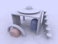
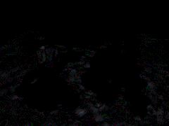
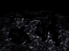
In most cases it is not necessary to change the low_error_factor. This factor reduces the error_bound value during the final pretrace step. pretrace_end was lowered to 0.01 in these pictures, the second line shows the difference to default. Changing this value can sometimes help to remove persistent artefacts.

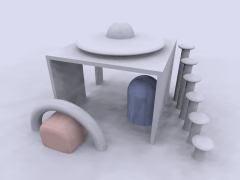
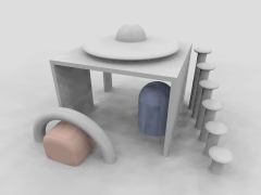
gray_threshold reduces the color in the radiosity calculations. as mentioned above the blue sky affects the color of the whole scene when radiosity is calculated. To reduce this coloring effect without affecting radiosity in general you can increase gray_threshold. 1.0 means no color in radiosity at all.

Another important parameter is pretrace_end. Together with pretrace_start it specifies the pretrace steps that are done. Lower values lead to more pretrace steps and more accurate results but also to significantly slower rendering.

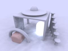
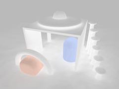
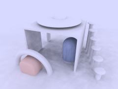
It is worth experimenting with the things affecting radiosity to get some feeling for how things work. The next 3 images show some more experiments.

ambient 3 instead of ambient 0 for one object

ambient 0.5 instead of ambient 0 for all objects sky: ambient 0

Finally you can strongly change the appearance of the whole scene with the sky's texture. The following pictures give some example.

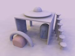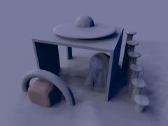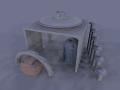Really good results mostly depends on the single situation and how the scene is meant to look. Here is some higher quality render of this particular scene, but requirements can be much different in other situations.

  global_settings {
    radiosity {
      pretrace_start 0.08
      pretrace_end   0.01
      count 500

      nearest_count 10
      error_bound 0.02
      recursion_limit 1

      low_error_factor 0.2
      gray_threshold 0.0
      minimum_reuse 0.015
      brightness 1

      adc_bailout 0.01/2
    }
  }

Normals and Radiosity

When using a normal statement in combination with radiosity lighting, you will see that the shadowed parts of the objects are totally smooth, no matter how strong the normals are made.

The reason is that POV-Ray by default does not take the normal into account when calculating radiosity. You can change this by adding normal on to the radiosity block. This can slow things down quite a lot, but usually leads to more realistic results if normals are used.

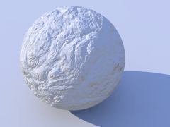
When using normals you should also remember that they are only faked irregularities and do not generate real geometric disturbances of the surface. A more realistic approach is using an isosurface with a pigment function, but this usually leads to very slow renders, especially if radiosity is involved.

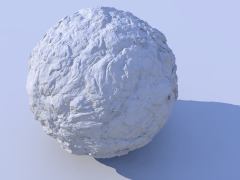You can see that the isosurface version does not have a natural smooth circumference and a more realistic shadowline.

Performance considerations

Radiosity can be very slow. To some extend this is the price to pay for realistic lighting, but there are a lot of things that can be done to improve speed.

The radiosity settings should be set as fast as possible. In most cases this is a quality vs. speed compromise. Especially recursion_limit should be kept as low as possible. Sometimes 1 is sufficient, if not 2 or 3 should often be enough.

With high quality settings, radiosity data can take quite a lot of memory. Apart from that the other scene data is also used much more intensively than in a conventional scene. Therefore insufficient memory and swapping can slow down things even more.

Finally the scene geometry and textures are important too. Objects not visible in the camera usually only increase parsing time and memory use, but in a radiosity scene, also objects behind the camera can slow down the rendering process.

Making Animations

There are a number of programs available that will take a series of still image files (such as POV-Ray outputs) and assemble them into animations. Such programs can produce AVI, MPEG, FLI/FLC, QuickTime, or even animated GIF files (for use on the World Wide Web). The trick, therefore, is how to produce the frames. That, of course, is where POV-Ray comes in. In earlier versions producing an animation series was no joy, as everything had to be done manually. We had to set the clock variable, and handle producing unique file names for each individual frame by hand. We could achieve some degree of automation by using batch files or similar scripting devices, but still, We had to set it all up by hand, and that was a lot of work (not to mention frustration... imagine forgetting to set the individual file names and coming back 24 hours later to find each frame had overwritten the last).

Now, at last, with POV-Ray 3, there is a better way. We no longer need a separate batch script or external sequencing programs, because a few simple settings in our INI file (or on the command line) will activate an internal animation sequence which will cause POV-Ray to automatically handle the animation loop details for us.

Actually, there are two halves to animation support: those settings we put in the INI file (or on the command line), and those code modifications we work into our scene description file. If we have already worked with animation in previous versions of POV-Ray, we can probably skip ahead to the section INI File Settings below. Otherwise, let's start with basics. Before we get to how to activate the internal animation loop, let's look at a couple examples of how a couple of keywords can set up our code to describe the motions of objects over time.

The Clock Variable: Key To It All

POV-Ray supports an automatically declared floating point variable identified as clock (all lower case). This is the key to making image files that can be automated. In command line operations, the clock variable is set using the +k switch. For example, +k3.4 from the command line would set the value of clock to 3.4. The same could be accomplished from the INI file using Clock=3.4 in an INI file.

If we do not set clock for anything, and the animation loop is not used (as will be described a little later) the clock variable is still there - it is just set for the default value of 0.0, so it is possible to set up some POV code for the purpose of animation, and still render it as a still picture during the object/world creation stage of our project.

The simplest example of using this to our advantage would be having an object which is travelling at a constant rate, say, along the x-axis. We would have the statement

  translate <clock, 0, 0>

in our object's declaration, and then have the animation loop assign progressively higher values to clock. And that is fine, as long as only one element or aspect of our scene is changing, but what happens when we want to control multiple changes in the same scene simultaneously?

The secret here is to use normalized clock values, and then make other variables in your scene proportional to clock. That is, when we set up our clock, (we are getting to that, patience!) have it run from 0.0 to 1.0, and then use that as a multiplier to some other values. That way, the other values can be whatever we need them to be, and clock can be the same 0 to 1 value for every application. Let's look at a (relatively) simple example

  #include "colors.inc"
  camera {
    location <0, 3, -6>
    look_at <0, 0, 0>
  }
  light_source { <20, 20, -20> color White }
  plane {
    y, 0
    pigment { checker color White color Black }
  }
  sphere {
    <0, 0, 0> , 1
    pigment {
      gradient x
      color_map {
        [0.0 Blue  ]
        [0.5 Blue  ]
        [0.5 White ]
        [1.0 White ]
      }
      scale .25
    }
    rotate <0, 0, -clock*360>
    translate <-pi, 1, 0>
    translate <2*pi*clock, 0, 0>
  }

Assuming that a series of frames is run with the clock progressively going from 0.0 to 1.0, the above code will produce a striped ball which rolls from left to right across the screen. We have two goals here:

Translate the ball from point A to point B, and,
Rotate the ball in exactly the right proportion to its linear movement to imply that it is rolling -- not gliding -- to its final position.

Taking the second goal first, we start with the sphere at the origin, because anywhere else and rotation will cause it to orbit the origin instead of rotating. Throughout the course of the animation, the ball will turn one complete 360 degree turn. Therefore, we used the formula, 360*clock to determine the rotation in each frame. Since clock runs 0 to 1, the rotation of the sphere runs from 0 degrees through 360.

Then we used the first translation to put the sphere at its initial starting point. Remember, we could not have just declared it there, or it would have orbited the origin, so before we can meet our other goal (translation), we have to compensate by putting the sphere back where it would have been at the start. After that, we re-translate the sphere by a clock relative distance, causing it to move relative to the starting point. We have chosen the formula of 2*pi* r*clock (the widest circumference of the sphere times current clock value) so that it will appear to move a distance equal to the circumference of the sphere in the same time that it rotates a complete 360 degrees. In this way, we have synchronized the rotation of the sphere to its translation, making it appear to be smoothly rolling along the plane.

Besides allowing us to coordinate multiple aspects of change over time more cleanly, mathematically speaking, the other good reason for using normalized clock values is that it will not matter whether we are doing a ten frame animated GIF, or a three hundred frame AVI. Values of the clock are proportioned to the number of frames, so that same POV code will work without regard to how long the frame sequence is. Our rolling ball will still travel the exact same amount no matter how many frames our animation ends up with.

Clock Dependant Variables And Multi-Stage Animations

Okay, what if we wanted the ball to roll left to right for the first half of the animation, then change direction 135 degrees and roll right to left, and toward the back of the scene. We would need to make use of POV-Ray's new conditional rendering directives, and test the clock value to determine when we reach the halfway point, then start rendering a different clock dependant sequence. But our goal, as above, it to be working in each stage with a variable in the range of 0 to 1 (normalized) because this makes the math so much cleaner to work with when we have to control multiple aspects during animation. So let's assume we keep the same camera, light, and plane, and let the clock run from 0 to 2! Now, replace the single sphere declaration with the following...

  #if ( clock <= 1 )
    sphere { <0, 0, 0> , 1
      pigment {
        gradient x
        color_map {
          [0.0 Blue  ]
          [0.5 Blue  ]
          [0.5 White ]
          [1.0 White ]
        }
        scale .25
      }
      rotate <0, 0, -clock*360>
      translate <-pi, 1, 0>
      translate <2*pi*clock, 0, 0>
    }
  #else
    // (if clock is > 1, we're on the second phase)
    // we still want to work with  a value from 0 - 1
    #declare ElseClock = clock - 1;
    sphere { <0, 0, 0> , 1
      pigment {
        gradient x
        color_map {
          [0.0 Blue  ]
          [0.5 Blue  ]
          [0.5 White ]
          [1.0 White ]
        }
        scale .25
      }
      rotate <0, 0, ElseClock*360>
      translate <-2*pi*ElseClock, 0, 0>
      rotate <0, 45, 0>
      translate <pi, 1, 0>
    }
  #end

If we spotted the fact that this will cause the ball to do an unrealistic snap turn when changing direction, bonus points for us - we are a born animator. However, for the simplicity of the example, let's ignore that for now. It will be easy enough to fix in the real world, once we examine how the existing code works.

All we did differently was assume that the clock would run 0 to 2, and that we wanted to be working with a normalized value instead. So when the clock goes over 1.0, POV assumes the second phase of the journey has begun, and we declare a new variable Elseclock which we make relative to the original built in clock, in such a way that while clock is going 1 to 2, Elseclock is going 0 to 1. So, even though there is only one clock, there can be as many additional variables as we care to declare (and have memory for), so even in fairly complex scenes, the single clock variable can be made the common coordinating factor which orchestrates all other motions.

The Phase Keyword

There is another keyword we should know for purposes of animations: the phase keyword. The phase keyword can be used on many texture elements, especially those that can take a color, pigment, normal or texture map. Remember the form that these maps take. For example:

  color_map {
    [0.00 White ]
    [0.25 Blue ]
    [0.76 Green ]
    [1.00 Red ]
  }

The floating point value to the left inside each set of brackets helps POV-Ray to map the color values to various areas of the object being textured. Notice that the map runs cleanly from 0.0 to 1.0?

Phase causes the color values to become shifted along the map by a floating point value which follows the keyword phase. Now, if we are using a normalized clock value already anyhow, we can make the variable clock the floating point value associated with phase, and the pattern will smoothly shift over the course of the animation. Let's look at a common example using a gradient normal pattern

  #include "colors.inc"
  #include "textures.inc"
  background { rgb<0.8, 0.8, 0.8> }
  camera {
    location <1.5, 1, -30>
    look_at <0, 1, 0>
    angle 10
  }
  light_source { <-100, 20, -100> color White }
  // flag
  polygon {
    5, <0, 0>, <0, 1>, <1, 1>, <1, 0>, <0, 0>
    pigment { Blue }
    normal {
      gradient x
      phase clock
      scale <0.2, 1, 1>
      sine_wave
    }
    scale <3, 2, 1>
    translate <-1.5, 0, 0>
  }
  // flagpole
  cylinder {
    <-1.5, -4, 0>, <-1.5, 2.25, 0>, 0.05
    texture { Silver_Metal }
  }
  // polecap
  sphere {
    <-1.5, 2.25, 0>, 0.1
    texture { Silver_Metal }
  }

Now, here we have created a simple blue flag with a gradient normal pattern on it. We have forced the gradient to use a sine-wave type wave so that it looks like the flag is rolling back and forth as though flapping in a breeze. But the real magic here is that phase keyword. It has been set to take the clock variable as a floating point value which, as the clock increments slowly toward 1.0, will cause the crests and troughs of the flag's wave to shift along the x-axis. Effectively, when we animate the frames created by this code, it will look like the flag is actually rippling in the wind.

This is only one, simple example of how a clock dependant phase shift can create interesting animation effects. Trying phase will all sorts of texture patterns, and it is amazing the range of animation effects we can create simply by phase alone, without ever actually moving the object.

Scattering media

Do Not Use Jitter Or Crand