User:Le Forgeron

I use this page to pre-document some experimental code (as experimental, not distributed in official release)

Interesting documents & link

They should not be incorporated as such in the documentation, but can provide some interesting informations

Splines

Imported from Megapov
Relicensing from ABX is needed before allowing distribution
(some bugs get fixed in the process)

Also check the megapov documentation for better explanation or clarification.

Accessing splines data

Not only the value of a spline can be evaluated with the traditional SPLINE_IDENTIFIER ( FLOAT [, SPLINE_TYPE] ), it is also possible to get back the actual pieces of information from a spline.

dimension_size( SPLINE_IDENTIFIER ) provides the number of entries in the spline.

For each entry, the spline can be accessed like an array, the first element is the float of the path list and the second element the associated vector.

SPLINE_IDENTIFIER[ INDEX ][0] is a float
SPLINE_IDENTIFIER[ INDEX ][1] is a vector
INDEX should evolve as an integer from 0 to dimension_size(SPLINE_IDENTIFIER)-1

Additional types of splines

Sor spline

the curve followed by a sor can be evaluted by a spline of sor_spline type with a bit of manipulation: the y value of the sor must be used as the float of the path, and the x value become one of the component of the vector. The component of the vector never get negative with a sor spline.

spline{
   sor_spline
  -1.000000,0.000000*x
   0.000000,0.118143*x
   0.540084,0.620253*x
   0.827004,0.210970*x
   0.962025,0.194093*x
   1.000000,0.286920*x
   1.033755,0.468354*x
}

sor{
  7
  <0.000000, -1.000000>
  <0.118143,  0.000000>
  <0.620253,  0.540084>
  <0.210970,  0.827004>
  <0.194093,  0.962025>
  <0.286920,  1.000000>
  <0.468354,  1.033755>
}

akima spline

That spline will go through all its points, smoothly.

spline {
  akima_spline
  time_Val_1, <Vector_1> [,]
  time_Val_2, <Vector_2> [,]
    ...
  time_Val_n, <Vector_n>
}

tcb spline

Also know as Kochanek-Bartels spline, tcb stand for tension, continuity and bias.

The first and last point of such spline are not reached.

spline {
  tcb_spline [TCB_PARAMETERS]
  time_Val_1 [TCB_PARAMETERS], <Vector_1> [TCB_PARAMETERS][,]
  time_Val_2 [TCB_PARAMETERS], <Vector_2> [TCB_PARAMETERS][,]
    ...
  time_Val_n [TCB_PARAMETERS], <Vector_n> [TCB_PARAMETERS]
}

TCB_PARAMETERS:
  [tension FLOAT] [continuity FLOAT] [bias FLOAT]

The tension, continuity and bias are fully optional. Depending on the place where they appear, they control the spline in different ways:

Placed right after the tcb_spline keyword, they set the default values for all ends of the spline segments. This placement is ignored in case of copying spline without adding new controls because previous defaults were already propagated to each side of control points.
Placed between the time_value and the corresponding vector, the tcb parameters determine the properties of the spline segment ending in the vector that follows these parameters (as well as for the spline segment beginning at this vector if not overriden with the third position).
For tcb parameters following a vector, the properties of the spline segment beginning after this vector are set.

What is controlled by these parameters?

tension controls how sharply the curve bends.
continuity controls how rapid speed and direction change.
bias controls the direction of the curve as it passes through the control point.

x splines

X-Splines are an alternative to traditional splines that was introduced by Carole Blanc and Christophe Schlick in 1995.

XSplines have the very nice property that they can interpolate (go through) a control point as well as just approximate it. Sharp edges are also possible, but the curve is always C2 continuous, hence the sharp edges are only possible when the first derivative drops to zero.

An X-Spline is completely defined by a set of control point (vertices) and a set of parameters. One parameter is associated with each control point.

There is 3 variations of x splines:

basic
extended
general

basic x spline

The first and last point of such spline are not reached.

spline {
  basic_x_spline [freedom_degree FLOAT]
  time_Val_1, <Vector_1> [,]
  time_Val_2, <Vector_2> [,]
  ...
  time_Val_n, <Vector_n>
}

extended x spline

general x spline

Colour space interpolation

The colour interpolation is available for:

mesh
blob
polygon

It can be used with texture_map, pigment_map or colour_map.

The interpolation is performed between the resulting colours from the evaluation, not along the map.

Which colourspace ?

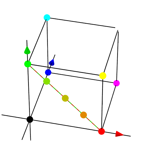
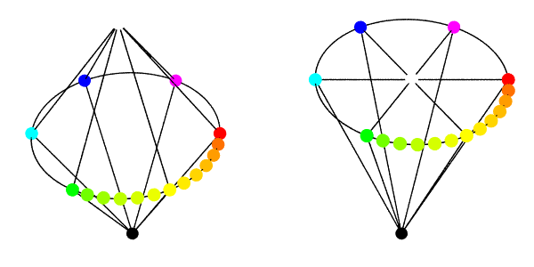
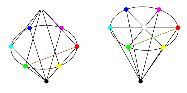
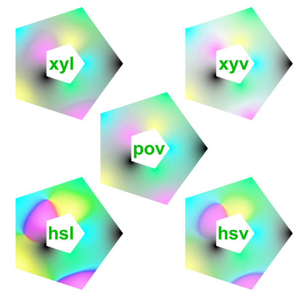
colour_space pov
colour_space hsl
colour_space hsv
colour_space xyl
colour_space xyv

color_space is also a valid synonym for colour_space.

pov

Classical linear interpolation in the rgb space.

50% of pure Red (rgb <1, 0, 0>) and pure Green (rgb <0, 1, 0 >) is a dark yellow (rgb <1/2, 1/2, 0>).

hsl or hsv

The colour (from rgb space) is converted to the HSL ot HSV colour system where the linear interpolation is performed.

50% of pure Red and pure Green turns out as pure Yellow.

xyl or xyv

the hs part is considered as polar coordinates (h, hue, being the angle and s being the length) of a point. The interpolation is performed using the Cartesian coordinates (xy).

The interpolation for the l or v part remains unchanged, a simple linear interpolation.

Mesh

Only one colour space per mesh, used for all its triangles.

mesh {
	triangle {0,x,y texture_list { colo1, colo2, colo3 } }
        ...
	colour_space hsv
}

blob

Only one colour space per blob, used for all components.

blob {
  ...	
   	colour_space hsv
}

Interpolation for polygon

a texture_list can be provided in the polygon, with a texture identifier for each vertex (and ignoring repeated vertex which are used to close a line)

The colour of any point from the polygon is a weighted average of each vertex, with the weight based on the distance to the vertex: the closer to a vertex, the more weight that vertex has. strength (with a float) can be used to adjust the relative weight by raising them to the power of the strength: strong strength gives more pronounced partitions.

#declare colo3=texture { pigment {color rgb<0.,0.,0>}};
#declare colo4=texture { pigment {color rgb<0.,1.,1/3>}};
#declare colo5=texture { pigment {color rgb<0.,1.,1>}};
#declare colo6=texture { pigment {color rgb<1.,1.,1/3>}};
#declare colo7=texture { pigment {color rgb<1.,1./3,1>}};
#declare num=5;
#declare step=2;
                                polygon { (num+1)*step,
#local j=0.70;
#while(j>0.1)
#local i=0;
#while(i<num+1)
		                j*< cos(i*2*pi/num),sin(i*2*pi/num),0>
#local i=i+1;
#end
#local j=j-0.90/step;
#end
			texture_list { colo3, colo4, colo5, colo6, colo7, colo5, colo6, colo7, colo3, colo4 } 
                        strength 1.0
}

colour_space is of course available too.

Access to camera information

These pieces of information are in read-only mode. You cannot use them to modify the actual value (no #declare or #local). The various vectors might have been updated by transform and look_at.

camera_type is a string containing the type of the camera (but not its subtype, so cylinder camera might be ambiguous).
camera_up is the actual up vector of the camera.
camera_right is the actual right vector of the camera.
camera_direction is the actual direction vector of the camera.

In case of scene with multiple cameras, each keyword can be followed by an usual array notation to access the relevant camera. (e.g. camera_up[3] for the fourth camera)

Tesselation & mesh play

Yoda: Yes, run! Yes, a Jedi's strength flows from the Renderer. But beware of the dark side. 
      Mesh, Heightfield, Bicubic Patch; the dark side of the Force are they. Easily they flow, 
      quick to join you in a fight. If once you start down the dark path, 
      forever will it dominate your destiny, consume you it will, as it did Isosurface's apprentice.
Luke: Parametric precompute... Is the dark side stronger?
Yoda: No, no, no. Quicker, easier, more seductive.
Luke: But how am I to know the good side from the bad?
Yoda: You will know... when you are calm, at peace, passive. 
      A Jedi uses the Renderer for knowledge and defense, NEVER for attack.
Luke: But tell my why I can't...
Yoda: No, no! There is no "why".

Mesh from 3D finite object

it must be 3D, to have an inside test which is meaningfull
it must be finite, because the bounding box is use to specify the volume which will be sampled

Whatever the method used (it will always end as a mesh object, or inside a mesh object). there is some common parameters:

original is followed by the object to sample. It is really mandatory.
accuracy is followed by a 3D vector which specify the number of slices in each direction (it defaults to 10)
offset is followed by a float which move outward the position of each face of the bounding box used for scanning (default to 0, so beware of very tight perfect bounding box)

Without texture, using only Inside test (fast)

These approaches use a marching cube algorithm, hence their usage were forbidden on the USA thanks to a now expired patent (17 years after December 1987).

bourke ( inspired by Paul Bourke at http://local.wasp.uwa.edu.au/~pbourke/geometry/polygonise/ , named with explicit authorisation)
heller ( alternate table from Bourke page made by Geoffrey Heller)
cubicle (simplistic approach using a cube)
cristal (same as cubicle, with inclined face)

bourke & heller allow an additional precision option, with a float, which supersample along the interecting line (by the amount of the float, so only positive integer are of any real interest) for a better fit.

Using Inside test & trace (slower)

No marching cube per itself here, the inside test is used to trigger the usage of trace to get the actual intersection.

tesselate

tessel

As trace is used, the texture from the intersection point is available and can be pushed on the vertex of each generated triangle.

a possible parameter is smooth which would also use the normal reported by the intersection to make smooth_triangle instead of triangle in the resulting mesh.

Mesh from and to file

Loading

A GTS file can be loaded with gts_load.

#include "colors.inc"
camera { location <3,5,-4>
	direction z
		up y
		right image_width/image_height*x
		look_at <-1/2,1/2,0>
		angle 35
}

light_source{ <-5, 20, -20>, 1}
light_source{ <0, 2, 0>, 1/2}

gts_load{ "bunny.gts"
	right
	rotate 180*y	
	scale 17
	translate -2*y
	texture { pigment { color Aquamarine}}
}

Aside from the filename of the file to load, the right keyword can be used to change the default left-handed coordinate system to a right-handed one.

gts_load can be used to create a mesh of its own or to incorporate the mesh of the file into a larger mesh, in which case a texture identifier can be applied over the loaded GTS mesh.

 mesh { ...
    gts_load { filename [right] [texture { Tid }] ... }
  ...
 }

OR

 gts_load { filename [right] ... }

Saving

A mesh can be saved with gts_save. Beware of I/O restrictions.

gts_save { filename, mesh_object }

GTS format saves the geometry, but neither the faked normal or the textures

Getting a new mesh from a mesh

The following method (or pseudo-object) can be used only on a mesh, whatever its origin.