Note! While the following density_file (.df3) pattern documentation is often valid with respect to the current 3.7.0 forms of df3 value interpolation, it is written as if the additional interpolation modes proposed in https://github.com/wfpokorny/povray/tree/feature/newDensityPatternInterpolations have been adopted for the 3.7.1 release.

Density File Pattern

The density_file pattern is a 3-D bitmap pattern that occupies a unit cube from location <0,0,0> to <1,1,1>. The data file is a raw binary file format created for POV-Ray called the df3 format. This pattern was originally created for use with halo or media, but it may be used anywhere a pattern may be used. The core syntax whether used in a normal, pattern or pigment block is:

density_file df3 [file name] [interpolate Type]

where the file name would be placed in double quotes and the interpolation type would be an integer value 0 through 12. For example:

density_file df3 "star.df3" 1

The general forms for each of the normal, pattern and pigment blocks are:

normal {
  density_file df3 [filename] [,Bump_Size]
  [interpolate Type]
  [NORMAL_MODIFIERS...]
}

where Bump_Size is an optional float value,

pattern {
  density_file df3 [filename] [interpolate Type]
  [PATTERN_MODIFIERS...]
}

and

pigment {
  density_file df3 [filename] [interpolate Type]
  [PIGMENT_MODIFIERS...]
}

The df3 file format

The df3 format consists of a 6 byte header of three 16-bit, unsigned integers with high order bytes first (big-endian order). These three values give the x,y,z size of the data in voxels.

The header is followed by x*y*z unsigned, big-endian encoded, integers with resolutions of 8, 16 or 32 bits. The resolution of the data is determined by the size of the df3 file. That is, if the file - minus the header - is twice as long as an 8 bit file, it is taken to contain 16 bit data. If it is four times as long, it is taken to contain 32 bit data.

How the density_file pattern works

The density pattern occupies the unit cube <0,0,0> to <1,1,1> regardless of the x, y, z dimensions in voxels. It remains at 0.0 for all areas beyond the unit cube. Data values in the ranges of 0 to 255 (8 bit/1 byte), 0 to 65535 (16 bit/2 bytes) and 0 to 4294967295 (32 bit/4 bytes), are scaled by the various interpolation methods to a float value in the range 0.0 to 1.0. The larger 2 byte and 4 byte depths providing better resolution.

There are currently thirteen data interpolation types numbered 0 through 12, with the types larger than 2 being available only in releases 3.7.1 and later. If nothing is specified via the interpolate keyword, the default is 0 which does no interpolation - meaning for a given location in the unit cube, the 0.0 to 1.0 value of the containing voxel is returned. The other interpolation methods available are:

Tri-linear. Similar to two dimensional image method, but for three dimensions.
Tri-cubic. Similar to two dimensional image method.
Weak exponential blobbing of defined voxels in 4x4x4 local sub regions.
Moderate exponential blobbing of defined voxels in 6x6x6 local sub regions.
Strong exponential blobbing of defined voxels in 8x8x8 local sub regions.
Spherical density, center to sides, within the density_file unit cube coordinate space. Specific coordinates of <+1.0e17,-1.0e17,-1.0e17>, < -1.0e17,+1.0e17,-1.0e17> and <-1.0e17,-1.0e17,+1.0e17> return the x, y and z df3 ranges as the ratio of the df3's range to the maximum, pow(2,16), range.
Gradient in x within the unit cube.
Gradient in y within the unit cube.
Gradient in z within the unit cube.
Returns x coordinate needed to rotate about unit cube's center y axis (lathe). Works too as a dual x,z gradient.
Returns x coordinate needed to twist about unit cube's center z axis one (twist left) rotation.
Returns y coordinate needed to twist about unit cube's center z axis one (twist left) rotation.

If an interpolate value not supported is specified, the interpolation defaults to tri-cubic interpolation, 2, in POV-Ray versions 3.6 and later.

Exponential blobbing interpolations.

Exponential blobbing techniques in POV-Ray date to the introduction of isosurface objects. The method here borrows from one common technique with the form:

1/exp((function's value)*(blobbing strength))

As implemented, for each evaluated point in the unit cube, the code sums the result of the equation:

(1/exp(pow(point_to_voxel_distance,2)*(internalTuningBias/voxel_value))

for all adjacent df3 values >0 within the NxNxN sub-cube around the evaluated point. Resulting values >1 are clamped to 1.0. The larger the sub cube, the stronger the blobbing which can be accommodated.

The algorithm has been tuned so 1.0 values for each of the exponential blobbing interpolations just fit within the corresponding sub cube. The blobbing can be adjusted without the need to regenerate a df3 by using the standard pattern wave modifier poly_wave <float>. Poly_wave values >=1.0 should always work and reduce the blobbing. Values < 1.0 increase the blobbing and can cause sub cube overruns. Overruns will appear as discontinuities in the final pattern.

A note on a possible extension to the density_file exponential blobbing methods. These today are based upon the square of the distance to nearby voxels with a value >0.0 and a strength blobbing factor based upon the value of those >0.0 voxels. When blobbing, the deeper 2 byte and 4 byte df3 formats are not often used. It is possible, with the 2 byte and 4 byte depths, to use 1 byte for the blobbing strength factor, and the remaining byte(s) to offset the evaluated voxel center for the distance squared component. At the 32 bit depth there would be 8x8x8 or 512 possible sub-voxel positions. Unsure of the ultimate performance for such code, the modeling/creating of df3s is certainly less straight forward, and such a method would be restricted to sparse data representations. Up to a 3x3x3, same weight (1/32 accuracy), bit representation at the 32 bit depth would be available too, if density of voxels were the aim.

Interpolations 6 through 12.

Interpolation 6 is internally called environment. It works in two different modes. In the first, using specific positive and negative values, it returns a density_file pattern df3's internal x, y and z range as the ratio of the range to the maximum allowed range. In the second, it returns a spherical gradient running from 1.0 at the 0.5,0.5,0.5 center of the unit cube to 0.0 at the unit cubes' sides. In general this latter mode is very like the spherical pattern, but with the significant advantage that no special set up is required for it to always be aligned with the density_file pattern based upon a df3 file.

Interpolations 6-12 are better thought of as density_file assist interpolations. Interpolation 10 wraps the >0.5 to 1.0 range in x about the y axis at a specific z value. Interpolations 11 and 12 provide x an y adjusted values to twist left about +z one rotation in the unit cube.

Note. The rotation and twist coordinates will clip at the unit cube corners as they rotate out of the unit cube's spatial frame. In other words, keep the data within a unit cube's center to side distance - away from the corners - unless trying for some clipped effect.

Only interpolation 0 is voxel centered in 3.7.0 and earlier releases.

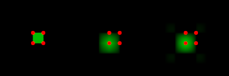
For version 3.7.0, the interpolations 0 to 2 are shown below in order, left to right, as a pigment on a plane for an 11x11x11 df3 file where a single center voxel has a value of 0.5 while all others are 0.0. The red dots mark the vertices around our center voxel.

Density_file interpolations for single center voxel as a green pigment on a plane with release 3.7.0.

The tri-linear and tri-cubic interpolations are vertex centered prior to 3.7.1 resulting in a half voxel negative shift in x,y,z . This shift is perhaps of no consequence if rendering media. It does however matter if, for example, building a df3 based isosurface or when trying to control textures for media for any formed objects using interpolation 0.

Offset tri-linear and tri-cubic results can be centered with a positive translation of one half a voxel size in x,y and z. For the 11x11x11 df3 example use:

translate <-0.5+(1/11/2),-0.5+(1/11/2),-0.5+(1/11/2)>

to get the density_file pattern exactly centered upon the origin. In a function for an isosurface this adjustment to center on the origin would be something like:

FnctAdjustToCenter(x+0.5-(1/11/2),y+0.5-(1/11/2),z+0.5-(1/11/2))

Release 3.7.1 makes all interpolations voxel, and so too unit cube, centered.

In addition to adding density_file pattern interpolation modes, 3.7.1 centers all the interpolated results. The 3.7.1 interpolations 0 to 5 are shown in order, left to right, in the following image.

Density_file interpolations for single center voxel as a green pigment on a plane.

Tri-linear interpolation has creases, tri-cubic interpolation wobbles/rings.

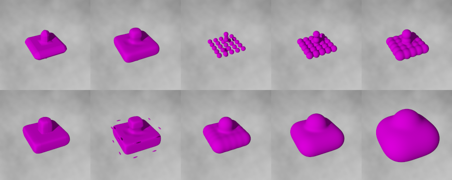
The following figure shows isosurfaces for interpolations 1 through 5, left to right, setting the threshold very near zero to better see the non-zero values returned. The df3 used is a 15x15x15 arrangement where an x,z box has been centered in y and through which there is a y column of >0.0 values. The values for the non-zero voxels in the top row are 0.1 and the bottom row 0.9.

The former better showing the crease effect of tri-linear interpolation, the latter, the ring of tri-cubic interpolation. The tri-cubic mode always wobbles, but the most severe artifacts can be avoided by using values not near 0.0 and 1.0 where pattern clipping occurs.

Density_file interpolations 1-5 for defined voxels arranged as box on spindle.

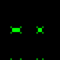
Lastly, with respect the the ringing of the tri-cubic interpolation, there are at times, additional harmonics as shown at the bottom of the following image which has been gamma adjusted to make this clear. The df3 sets only 3 voxels, here seen as the brighter green rectangles.

Density_file second ring example with tri-cubic interpolation.

DF3 value and density_file interpolation effects on an isosurface max gradient.

Interpolation methods and df3 values affect the max gradient in isosurface use. For tri-linear and tri-cubic Interpolations 1 and 2, lower values result in lower gradients due the typically longer ramp from the >0 edge to the voxel value used as a threshold. With the exponential blobbing of modes 3, 4 and 5, the lower gradients happen instead at larger voxel values - lower voxel values result in small spheres with much sharper local gradients. Gradients for interpolations 0-5 tend to increase as the df3 file's voxel count increase.

Interpolations 3, 4 and 5 max values always go to 1.0 at any >0.0 voxel center, where interpolations 1 and 2 peak at the voxel's specified >0.0 value.

Reported maximum gradients for df3 based isosurfaces will often be much higher than what can be used. These higher gradients occur where a ray catches the far corner or edge of the df3-function in a direction more perpendicular to the best overall local gradient. Note. This far corner, near threshold, gradient effect happens with other patterns too and can often be ignored in practice.

Use a buffer of five 0.0 voxels on all sides to avoid density_file edge effects.

While not a hard and fast rule, all the interpolations other than 0, and 6-12, will wrap or repeat values on the sides. The general recommendation of five comes from interpolation five's need for an 8 grid range (4 per side) about any evaluated point - plus a half voxel grid for the internal vertex to voxel center correction of interpolations 1-5. Often smaller buffer amounts can be used.

Below are two images. In the first, the lower-left-forward corner of the df3 has been filled with 0.2 values with all others 0.0. In the second image the top-right-back corner of df3 file has been set to values of 0.2 with all others set to 0.0. Interpolations 0 through 5 are shown left to right in each of these two images as a pigment on an x,y plane at the df3 unit cube's z center.

(1) Density_file interpolations 0-5 with defined left, bottom, front voxels.

(2) Density_file interpolations 0-5 with defined right, top, back voxels.

All truncate sharply to 0.0 where values have been run to the unit cube sides. This abrupt change is especially inconvenient for isosurface use, but the hard edge can often be seen in other pattern uses as some artifact.

The tri-linear and tri-cubic interpolations, 1 and 2, wrap side to opposite side in the lower-left-forward side-abutted case shown in the first row. These same interpolations truncate in the rop-right-back side-abutted case shown in the second row.

The exponential blobbing of 3 through 5 all repeat - or add values - at the last voxel position at the sides. This can sometimes be compensated for by lowering the on side and in-corner values.

User:Wfpokorny/DensityFile

Contents